Electromagnetic Pre-earthquake Precursors: Mechanisms, Data and Models-A Review
Received: 16-Nov-2014 / Accepted Date: 03-Jan-2015 / Published Date: 12-Jan-2015 DOI: 10.4172/2157-7617.1000250
Abstract
This paper is a survey of pre-earthquake short-term electromagnetic precursors. Extensive studies were carried out the last decades in analysis of electromagnetic emissions from 10-3 Hz up to MHz. These signals were analyzed through visual, statistical and chaotic techniques. The paper presents cumulative elements from scientific investigations performed during the last 40 years in this area. Physical models have also been developed for the interpretation of production and propagation of electromagnetic radiation during the fracture process. The Ultra Low Frequency (ULF) fracture-re-lated emissions attempted to be explained via magneto-hydrodynamic, piezomagnetic and electroki-netic effects whereas for the kHz-MHz observations the model of asperities was proposed.
Keywords: Electromagnetic emissions; Earthquake precursors; Ultra low frequency
Introduction
Natural events like earthquakes, tsunamis and volcanic eruptions are inevitable. What makes these events more dangerous and disastrous is not that they are inevitable but that they are still extremely hard to predict. Therefore, it is one of the major challenges for the world scientific community to find a reliable seismic precursor. The researchers have started efforts in this direction a lot of decades ago. However, the problem of earthquake prediction remains unsolved. Precursors recorded for certain earthquakes indicate there is evidence that they can be used for forecasting. In case of an earthquake rupture, certain precursory activity can be expected, if the observation is made in the near vicinity of causative fracture. The problem of earthquake prediction consists of consecutive, step-by-step, narrowing of the time interval, space and magnitude ranges, where a strong earthquake should be expected [1]. Five stages of prediction are usually distinguished. The background stage provides maps with the territorial distribution of the maximum possible magnitude and recurrence time of destructive earthquake of different magnitudes. Four subsequent stages, fuzzily divided, include the time prediction; they differ in the characteristic time interval covered by an alarm. These stages are as follows [2]: longterm (101 years); intermediate-term (1 year); short-term (10-1 to 10-2 years), and immediate-term (10-3 years or less). Such division into stages is dictated by the character of the process that leads to a strong earthquake and by the needs of earthquake preparedness; the latter comprises an arsenal of safety measures for each stage of prediction [1]. According to Hayakawa and Hobara [3] the prediction of earthquakes is classified into three categories: long-term (timescale of 10 to 100 years); intermediate-term (time-scale of 1 to 10 years); short-term. Note, that even in short-term prediction there is no one-to-one correspondence between anomalies in the observations and the earthquake events [4,5]. Although much more difficult than the long-term and intermediateterm predictions, short-term prediction of earthquakes on a time-scale of hours, days or weeks, is believed to be of the highest priority for social demands in seismo-active countries.
The short-term earthquake precursors related with electromagnetic effects are promising tools for earthquake prediction. The subjective study of seismo-electromagnetism refers to electric and magnetic field anomalies [6] observed during seismicity. Various studies have shown that these pre-seismic electromagnetic emissions occur in wide frequency band ranging from few Hz to MHz. Global efforts to predict earthquakes were started about a century ago and peaked during 1970s. The first scientifically well documented earthquake prediction was made on the basis of temporal and spatial variation of ts/tp relation in Blue mountain Lake, New York on 3rd August, 1973 [7]. Seismologists then successfully predicted the M7.4 Heicheng China earthquake of February 4, 1975 (Cha Chi Yuan), which raised the hopes that it could be possible to make reliable earthquake forecasts. Because of this prediction, an alert was issued within the 24-hour period prior to the main shock, probably preventing a larger number of casualties than the 1328 deaths that actually occurred from this event. However, the failure to predict another devastating earthquake 18 months later, the 1976 M7.8 Tangshan earthquake, was a major setback to the earthquake prediction effort. Casualties from this earthquake numbered in the hundreds of thousands [8]. The seismologists have now narrowed down their studies from long term prediction to short term prediction [9]. The studies carried out in past three decades have given birth to the new field of seismo-electromagnetism. Several research groups all over the world have shown evidences of electromagnetic emissions and anomalies before earthquakes.
Despite the scientific efforts, the preparation and evolution of earthquakes is not delineated yet. A significant reason is that there is restricted knowledge of the fracture mechanisms of the crust [4,10-26]. This is reinforced by the fact that each earthquake is particular and happens in large-scale. Accounting that the fracture of heterogeneous materials is not sufficiently described yet, despite the tremendous upto- date effort at laboratory, theoretical and numerical level [4], it may be understood why the description of the genesis of earthquakes is still limited [4,10-26]. According to Eftaxias [4] one should expect that the preparatory processes of earthquakes have various facets, which may be potentially observed before the final catastrophe at geological, geochemical, hydrological and environmental scales [4].
In the following, significant scientific evidence is presented regarding forecasting of earthquakes. The analysis is limited to preearthquake electromagnetic disturbances considering these among the most credible precursors of general failure. Focus is mainly on shortterm precursors.
Short-term Forecasting Of Earthquakes-Problems And Limitations
The science of short-term earthquake prediction is the study of earthquake precursors. In fact, short-term predictions are typically based on observations of these types of phenomena. Earthquake precursors include serendipitous observations of physical processes ahead of at least some earthquakes [8]. These processes comprise detection of anomalies in electromagnetic fields, fluctuations in ground-water level, gas emissions, surface distortions due to pressure differences , changes in ionospheric parameters etc. [8]. It is important however to note that ULF, kHz and MHz EM anomalies have been detected over periods ranging from a few days to a few hours prior to recent destructive earthquakes that occurred in land or were strong and shallow [10-26]. Finally, it is the subject of seismo-electromagnetism to study electric and magnetic field anomalies observed during seismicity [6]. The related studies have reported pre-seismic electromagnetic emissions in wide frequency bands ranging from 0.001 Hz to MHz.
Two major criteria are significant in identifying earthquake precursors. The first criterion is to recognise credible scientific evidence regarding anomalies observed prior to earthquakes [4]. The successful measurement of some anomalous phenomenon prior to an earthquake usually depends on the luck of having a good scientific experiment operating in an area before, during and after an earthquake. The second criterion for the selection of the earthquake precursors is that there are accepted physical models to explain the existence of the precursor [8].
On the other hand, in material science and in geophysics, it is vital to identify precursors of macroscopic defects or shocks [4]. And this, because fracture induced physical fields allow real-time monitoring of damage evolution in materials during mechanical loading. A stressed rock behaves like a stress-electromagnetic transformer. The crack propagation is the basic mechanism of the failure of the material [20]. In many materials emission of photons, electrons, ions and neutral particles is observed during the formation of new surface features after fracturing, deformation, wearing, peeling etc. [18-22]. Collectively, these emissions are referred as fracto-emissions [20]. The rupture of inter-atomic (ionic) bonds also leads to intense charge separation that is the origin of the electric charge between the micro-crack faces. On the faces of a newly created micro-crack the electric charges constitute an electric dipole or a more complicated system. The motion of a crack has been shown to be governed by a dynamical instability causing oscillations in its velocity and structure on the fracture surface. Experimental evidence indicate that the instability mechanism is that of local branching: a multi-crack state is formed by repetitive, frustrated micro-fracturing events. It is worth mentioning that laboratory experiments show that more intense fracto-emissions are observed during the unstable crack growth [20,27-30]. Due to the strong wall vibration of cracks in the stage of the micro-branching instability, the fractured material behaves as an efficient electromagnetic emitter. Thus, when a material is strained, electromagnetic emissions in a wide frequency spectrum ranging from Hz to MHz are produced by opening cracks, which can be considered as the so-called precursors of general fracture. These electromagnetic precursors are detectable both at laboratory and geological scale [4,18-30]. In the above sense, it becomes evident that the main tool of the prediction of earthquakes is the monitoring of the micro-fractures, which possibly occur in the focal area before the final break-up, by recording their electromagnetic emissions [4].
Several investigations on earthquake prediction were based on visual observations. Numerous have utilized concepts from the theory of entropy and information [21,24,26,31]. Alternative approximations employed the use of fractal methods, symbolic dynamics, Natural Time, Hurst Exponent and DFA (Detrended Fluctuation Analysis) [4,10-33]. Usually employed entropy metrics were: [4,22,24,26,28] (i) Shannon entropy per letter (ii) Conditional entropy (iii) Entropy of the source (iv) T-entropy (v) Tsallis entropy (vi) Hurst exponent (vii) Fisher Information (viii) Perturbation entropy (ix) Fractal dimension. Pre-seismic EM precursors were investigated in terms of critical phenomena as well [16,19,22].
In the above sense, Table 1 presents a collection of relevant important data including: (1) earthquake details; (2) detected preearthquake disturbances; (3) detection techniques employed and analysis methods; (4) references from 1980 and after. It may be observed that most of the electromagnetic precursors are in ULF, LF and HF range. It may seen that the most disturbances were analyzed visually. Analysis based on advanced techniques has been reported in some cases. More significant seem to be the Natural Time and Detrended Fluctuation Analysis, the evolution of fractal dimension and Hurst exponent and the temporal changes of various metrics of entropy. The latter techniques investigated in detail, traces of long-memory hidden in pre-earthquake time-series or features of self-organization of the earthquake generating system.
| Earthquake | Disturbance | Detection | ||||||||
|---|---|---|---|---|---|---|---|---|---|---|
| Place | Magnitude | Date(s) | Emission type | Frequency range | Instrumentation | Method(s) | Precursory time | ED | Reference | |
| Single events | Chile | 10 | 22/05/1960 | Radio | 18 MHz | Radioastronomy receiver | Visual observation | b (6 days) | Worldwide | [34] |
| Hollister, California | 5.2 | 28/11/1974 | ULF magnetic | Array of 7 proton magnetometers | Visual observation | b(7week-several months) | 11 km | [35] | ||
| Tangshan, China | 7.8 | 28/07/1976 | Resistivity | Visual observation | b(2-3 years) | [36] | ||||
| Tangshan, China | 7.8 | 28/07/1976 | Self potential, magnetotelluric | Visual observation | b(3 months) | [36] | ||||
| Sungpan–Pingwu,China | 7.2 | 16/08/1976 | Telluric currents | Visual observation | b(1month) | [37] | ||||
| Sungpan–Pingwu,China | 6.8 | 22/08/1976 | Telluric currents | Visual observation | b(1month) | [37] | ||||
| Sungpan–Pingwu,China | 7.2 | 23/08/1976 | Telluric currents | Visual observation | b(1month) | [37] | ||||
| Kyoto, Japan | 7.0 | 31/03/1980 | LF electric | 81 kHz | Electric antenna | Visual observation | b(1/2 h) | 250 km | [38] | |
| Tokyo, Japan | 5.3 | 25/09/1980 | LF electric | 81 kHz | Electric antenna | Visual observation | b(1h) | 55 km | [38] | |
| Tokyo, Japan | 5.5 | 28/01/1981 | LF electric | 81 kHz | Electric antenna | Visual observation | b(3/4h) | 50 km | [38] | |
| Kalamata, Greece | 6.2 | 13/09/1986 | Electric | Visual observation | b(3-5days) | 200 km | [39] | |||
| Spitak, Armenia | 6.9 (Ms) | 07/12/1988 | ULF magnetic | 0.01-1Hz | 3-axis magnetometers | Visual observation & Statistical analysis | b(4h),a | 128 km | [6] | |
| Spitak, Armenia | 6.9 (Ms) | 07/12/1988 | ULF magnetic | 0.005-1Hz | Visual observation & Statistical analysis | b(4h).a | 120 km, 200 km | [40] | ||
| Loma Prieta, California | 7.1 (Ms) | 18/11/1989 | ULF magnetic | 0.01Hz | Visual observation & Statistical analysis | b(3h),a | 7 km | [6] | ||
| Loma Prieta, California | 7.1 (Ms) | 19/11/1989 | ELF-LF EM | 0.01Hz-32kHz | Ground-based magnetometers | Visual observation | b(3h),d | 52 km | [41] | |
| Spitak, Armenia | 6.9 (Ms) | 23/01/89 | ELF-LF EM | 140Hz,450 Hz 800Hz, 4500 Hz, 15000 Hz | COSMOS-1809 Satellite | Visual observation&StatisticalAnalysis&FFT | b(<3h) | Δlong<6°Δlat 2°-4°[12 from the 13 satelite orbits for f[42] | ||
| Upland, California | 4.3 | 17/04/1990 | ELF magnetic | 3-4Hz | Vertical magnetic sensor | Statistical Analysis&PSD-FFT | b(1d) | 160 km | [43] | |
| Western Iran | 7.5 | 20/06/1990 | Ionospheric(radiowave) | 0-8kHz,10-14kHz | INTERCOSMOS-19 satellite | Visual observation & Modelling | b(16d) | 250 km-2000 km | [44] | |
| Watsonville, California | 4.3 | 23/03/1991 | ELF magnetic | 3.0–4.0 Hz | North–south magnetic sensor | Statistical Analysis&PSD-FFT | b (data averaged over 2 days) | 600 km | [43] | |
| Watsonville, California | 4.3 | 23/03/1991 | ELF magnetic | 3.0–4.0 Hz | Vertical magnetic sensor | Statistical Analysis&PSD-FFT | b (data averaged over 2 days) | 600 km | [43] | |
| Coalinga, California | 4.0 | 15/01/1992 | ELF magnetic | 3.0–4.0 Hz | Vertical magnetic sensor | Statistical Analysis&PSD-FFT | b (data averaged over 2 days) | 400 km | [43] | |
| Hokkaido, Japan | 7.8 | 12/07/1993 | foF2 ionospheric | Visual observation & Statistical analysis | b (3 days) | 290 km, 780 km, 1280 km | [45] | |||
| Guam | 7.1 (Ms) | 8/8/1993 | ULF magnetic | 0.02–0.05 Hz | 3-axis ring–core-type ?uxgatemagnetometer (NS, EW, Vertical) | Fractal analysis with PSD-FFT | b (1 month) | 65 km | [46-48] | |
| Guam | 8.3 (MJAM) | 8/8/1993 | ULF magnetic | 0.02–0.05 Hz | 3-axis ring–core-type ?uxgatemagnetometer (NS, EW, Vertical) | MultifractalDetrended Fluctuation Analysis | b (1 month) | 65 km | [49] | |
| Hokkaido–Toho–Oki, Japn | 8.1 (MW) | 04/10/1994 | LF electric | Borehole antenna | Visual observation | b (20 min) | >1000 km | [50] | ||
| Hyogo-ken Nanbu (Kobe), Japan | 7.2 | 17/01/1995 | DC geopotential, ELF magnetic,LF radio, MF–HF, FM-wave | 223 Hzz, 1–20 kHz, 163 kHz, 77.1 MHz | Visual & statistical analysis | b (≥ 100 km[51] | ||||
| Hyogo-ken Nanbu (Kobe), Japan | 7.2 (M0) | 17/01/1995 | LF radio | 10.2 kHz | LF Omega transmitter and receiver | Statistical Analysis (TT method) & Modelling | b (2 days) | 70 km | [6] | |
| Hyogo-ken Nanbu (Kobe), Japan | 7.2 | 17/01/1995 | Electric | 22.2 MHz | Phase-switched interferometer with two horizontally-polarized antennas | b (1 h) | 77 km | [52] | ||
| Kozani-Grevena, Greece | 6.6 (MW) | 13/05/1995 | Electric, magnetic | b (2 weeks) | 70 m, 200 km | [53] | ||||
| Kozani-Grevena, Greece | 6.6 (MW) | 13/05/1995 | HF electromagnetic | E: 41 and 54 MHz M: 3 & 10 kHz | Electric dipole antennas, magnetic loop antennas | PSD-Wavelet Spestral Fractal analysis | b (20 h) | 284 km | [10,12] | |
| Kozani-Grevena, Greece | 6.6 (MW) | 13/05/1995 | HF electromagnetic | E: 41 and 54 MHz M: 3 & 10 kHz | Electric dipole antennas, magnetic loop antennas | PSD-Wavelet Spestral Fractal analysis and Statistical methods. | b (20 h) | 284 km | [13] | |
| Kozani-Grevena, Greece | 6.6 (MW) | 13/05/1995 | HF electromagnetic | E: 41 and 54 MHz M: 3 & 10 kHz | Electric dipole antennas, magnetic loop antennas | PSD-Wavelet Spestral Fractal analysis and Statistical methods. | b (20 h) | 284 km | [14] | |
| Kozani-Grevena, Greece | 6.6 (MW) | 13/05/1995 | HF electromagnetic | E: 41 MHz | Electric dipole antennas, magnetic loop antennas | PSD-Wavelet Spestral Fractal analysis and Statistical methods. | b (20 h) | 284 km | [15] | |
| Kozani-Grevena, Greece | 6.6 (MW) | 13/05/1995 | HF electromagnetic | E: 41 and 54 MHz M: 3 & 10 kHz | Electric dipole antennas, magnetic loop antennas | Intermittent dynamics of critical fluctuations (IDCF)-model & Approximation of Power Spectral Density | b (20 h) | 284 km | [55] | |
| Kozani-Grevena, Greece | 6.6 (MW) | 13/05/1995 | SES | ≤1 Hz | Electric dipole antennas, magnetic antennas | Visual and mathematical analysis | b (4 weeks) | 70 km-80 km | [56] | |
| Kozani-Grevena, Greece | 6.8 (Ms) | 13/05/1995 | SES | ≤1 Hz | Electric dipole antennas, magnetic antennas | Visual and mathematical analysis | b (24,25 days) | 70 km-80 km | [57] | |
| Kozani-Grevena, Greece | 6.8 (Ms) | 13/05/1995 | SES | ≤1 Hz | Electric dipole antennas, magnetic antennas | Visual and mathematical analysis | b (22 min-3min) | 70 km-80 km | [58] | |
| Mid Niigata prefecture | 6.8(MJMA) | 16/08/2005 | DC/ULF magnetic HF/LF | 0.02–0.05 Hz 40 kHz | 3-axis ring–core-type ?uxgatemagnetometer (NS, EW, Vertical) Discon-type antenna (from 25 MHz to 1300 MHz) with IC-RF75 HF reciever | Signal analysis with FFT | b (17-21 days & 5-7 days) | [59] | ||
| Miyagi-ken oki Japan | 7.2 (MW) | 16/08/2005 | HF electromagnetic | 49.5 MHz | Discon-type antenna (from 25 MHz to 1300 MHz) with IC-RF75 HF reciever | (Spectral slope estimation, multi-fractal detrended fluctuation analysis & multi-fractal wavelet transform modulus maxima method. | b (2-3 weeks & few days-Kunimi station only) | 90 km -140 km | [60] | |
| Akita-ken Nairiku-nanbu, Japan | 5.9 | 11/08/1996 | HF electric | 10 kHz- 1MHz | Vertical-dipole ground electrodes | Visual analysis and analysis of related parameters | b (6 days) | [51] | ||
| Chiba-ken Toho-oki, Japan | 6.6 | 11/09/1996 | HF electric | 10 kHz- 1MHz | Vertical-dipole ground electrodes | Visual analysis and analysis of related parameters | b (3 days) | 320 km, 430 km | [51] | |
| Umbria–Marche, Italy | 5.5 | 26/03/1998 | LF radio | 0.006 Hz | Radio wave vertical antenna | b (1.5 months) | 818 km | [61] | ||
| San Juan Bautista, California | 5.1 (MW) | 12/08/1998 | UHF magnetic | 0.01–10 Hz | 3-component magnetic ?eld inductor coils | Statistical analysis and Power spectrum analysis (MA indices) | b (2 h) | 3 km | [62] | |
| Athens, Greece | 5.9 (MW) | 07/09/1999 | LF electromagnetic | M: 3 & 10 kHz | Magnetic loop antennas | Delay Times Method, Approximate Entropy, Spectral Fractal Analysis | b (12-17 h) | 247 km | [63] | |
| Athens, Greece | 5.9 (MW) | 07/09/1999 | LF electromagnetic | M: 3 & 10 kHz | Magnetic loop antennas | Wavelet Power Spectrum analysis | b (12-17 h) | 247 km | [64] | |
| Athens, Greece | 5.9 (MW) | 07/09/1999 | LF electromagnetic | M: 3 & 10 kHz | Magnetic loop antennas | Symbolic Dynamics | b (12-17 h) | 247 km | [64] | |
| Athens, Greece | 5.9 (MW) | 07/09/1999 | HF & LF electromagnetic | E: 41 and 54 MHz M: 3 & 10 kHz | Electric dipole antennas, magnetic loop antennas | Wavelet Power Spectrum analysis | b (12-17 h) | 247 km | [10,12] | |
| Athens, Greece | 5.9 (MW) | 07/09/1999 | HF & LF electromagnetic | M: 10 kHz | Electric dipole antennas, magnetic loop antennas | Block Entropy, Kolmogorov-Sinai Entropy, Conditional Entropy | b (12-17 h) | 247 km | [65] | |
| Athens, Greece | 5.9 (MW) | 07/09/1999 | LF electromagnetic | M: 3 & 10 kHz | Magnetic loop antennas | Symbolic Dynamics | b (12-17 h) | 247 km | [64] | |
| Athens, Greece | 5.9 (MW) | 07/09/1999 | HF & LF electromagnetic | E:154 MHz M: 3 & 10 kHz | Electric dipole antennas, magnetic loop antennas | Intermittent dynamics of critical fluctuations (IDCF)-model &Approximation of Power Spectral Density | b (20 h) | 247 km | [55] | |
| Athens, Greece | 5.9 (MW) | 07/09/1999 | HF & LF electromagnetic | E: 135 MHz M:10 kHz | Electric dipole antennas, magnetic loop antennas | Intermittent dynamics of critical fluctuations (IDCF)-model & Hurst Analysis | b (>3 h) | 247 km | [55] | |
| Athens, Greece | 5.9 (MW) | 07/09/1999 | HF & LF electromagnetic | M: 10 kHz | Electric dipole antennas, magnetic loop antennas | Tsallis Entropy | b (12-17 h) | 247 km | [31] | |
| Athens, Greece | 5.9 (MW) | 07/09/1999 | HF & LF electromagnetic | M: 10 kHz | Electric dipole antennas, magnetic loop antennas | Statistical Analysis | b (12-17 h) | 247 km | [66] | |
| Athens, Greece | 5.9 (MW) | 07/09/1999 | HF & LF electromagnetic | M: 10 kHz | Electric dipole antennas, magnetic loop antennas | Tsallis Entropy & Fisher Information (10 kHz) | b (12-17 h) | 247 km | [24] | |
| Athens, Greece | 5.9 (MW) | 07/09/1999 | HF & LF electromagnetic | M: 10 kHz | Electric dipole antennas, magnetic loop antennas | T-Entropy & R/S analysis & wavelet spectral fractal analysis | b (12-17 h) | 247 km | [23] | |
| Athens, Greece | 5.9 (MW) | 07/09/1999 | HF & LF electromagnetic | 10 kHz | Electric dipole antennas, magnetic loop antennas | Fisher Information, Approximate Entropy | b (<3h) | 284 km | [67] | |
| Chi-Chi, Taiwan | 7.6 (MW) | 20/09/1999 | foF2 ionospheric | IPS-42 ionosonde | Visual observation | b (3-4 days) | 120 km | [68] | ||
| Chia-Yii, Taiwan | 6.4 (MW) | 22/10/1999 | foF2 ionospheric | IPS-42 ionosonde | Visual observation | b (1-3 days) | 179 km | [68] | ||
| L'Aquila, Italy | 6.3 | 06/04/2009 | HF & LF electromagnetic | E: 41 and 54 MHz M: 3 & 10 kHz | Electric dipole antennas, magnetic loop antennas | Wavelet Power Spectrum analysis,Block Entropy, Kolmogorov-Sinai Entropy, Conditional Entropy, Entropy of the source, approximate entropy, Tsallis entropy, normalisedTsallis entropy, T-entropy, DFA, R/S analysis, Hurst analysis, | b(<3h) | 816 km | [21,22] | |
| Multiple Events | Greece (3 events) | 6.0 [NW Crete] 5.0 [SE Crete] 5.0 [NE Samos] | 21/11/1992 29/07/1995 07/05/1995 | HF electromagnetic | E: 41 and 53 MHz | Electric dipole antennas | Visual observation | b (1-3 days) | 20-150 km | [69] |
| Greece (2 events) | 6.6(MW)[Kozani-Grevena] 6.6 (MW)[Athens] | 13//05/1995 07/09/1999 | ULF, HF & LF electromagnetic | SES 1Hz E: 41, 54 and 135 MHz M: 3 & 10 kHz | Electric dipole antennas, magnetic loop antennas | Wavelet Power Spectrum analysis, Symbolic Dynamics, T-Entropy, Approximate Entropy, normalisedTsallis Entropy, | b (284km, 247 km[18] | |||
| Greece (4 events) | 6.6(MW)[Kozani-Grevena] 5.9 (MW) [Egio-Eratini]6.6 (MW)[Athens] 5.9 (MW) [Lefkas] | 13//05/1995 15/06/1995 07/09/1999 14/06/2003 | HF & LF electromagnetic | E: 41 and 54 MHz M: 3 & 10 kHz | Electric dipole antennas, magnetic loop antennas | Wavelet Power Spectrum analysis, Symbolic Dynamics, T-Entropy, Approximate Entropy, normalisedTsallis Entropy, | b (12-17 h) | [17] | ||
| Japan (4 events) (swarm earthquakes of depth~10km) | 6.4 (MJMA) [Izu-Peninsula] 6.1 (MJMA) [Izu-Peninsula] 6.3 (MJMA) [Izu-Peninsula] 6.0 (MJMA) [Izu-Peninsula] | 01/07/2000 09/07/2000 15/07/2000 18/08/2000 | ULF geomagnetic | 0.001-1 Hz | 3-axis ring–core-type ?uxgatemagnetometer (NS, EW, Vertical) | Fractal analysis with FFT, Higuchi and Bulgara-Klein methods | b (80 km-1160 km[70] | |||
| Japan (5 events) | 8.3 (MJMA) [Guam] 6.4 (MJMA) [Izu-Peninsula] 6.1 (MJMA) [Izu-Peninsula] 6.3 (MJMA) [Izu-Peninsula] 6.0 (MJMA) [Izu-Peninsula] | 08/08/1993 01/07/2000 09/07/2000 15/07/2000 18/08/2000 | ULF geomagnetic | 0.001-1 Hz | 3-axis ring–core-type ?uxgatemagnetometer (NS, EW, Vertical) | Fractal analysis with FFT, Fractal Dimension | b (80 km-1160 km[71] | |||
| Greece (2 events) | 5.2 (ML) & 5.8 (ML) | 18/01/200& 03/02/2007 | SES | ≤1 Hz | Electric dipole antennas & Magnetic antennas | Natural time analysis | b (22min),a(3min) | [58] | ||
| Greece | Synthetic& 6.4 (MW) | 08/06/2008 | SES | ≤1 Hz | Electric dipole antennas & Magnetic antennas | Natural time analysis | [32] | |||
| Japan | 7.8 (MJMA) [SW offshore Hokkaido] 8.2 (MJMA) [E offshore Hokkaido] 7.6 (MJMA) [far-offshore Hokkaido] 8.0 (MsMA) [offshore Tokachi] 7.8 (MJMA) [Near Chichi-jima] 9.0 (MsJMA) [Tohoku] | 07/12/1993& 04/10/1994& 28/12/1994& 26/09/2003& 22/10/2010& 11/3/2011 | SES | ≤1 Hz | Electric dipole antennas& Magnetic antennas | Natural time analysis | b(1 month) [for Tohoku and remaining 6 major EQs with MJMA≥7.6, depthΔLat<3°Δlong<3°[33] | |||
| Sumatra, Indonesia | 9.0 (Mw) [Sumatra-Andaman] 8.7 (Mw) [Sumatra-Nias] | 26/12/2004 28/3/2205 | ULF geomagnetic | 1 Hz | 3-axis ring–core-type ?uxgatemagnetometer (NS, EW, Vertical) | Spectral density ratio analysis and transfer functions analysis based on wavelet transform method, fractal dimension. | b ([72] | |||
| Sumatra, Indonesia | 9.3 8.7 | 26/12/2004 28/3/2205 | Geomagnetic | 1 Hz | CHAMP satellite vector magnetic antennas | Wavelet Power Spectrum analysis | b(few hours),a(2 hours) | 700 km region | [25] | |
| Seismic Periods | Worldwide (325 events) | > 5 (Ms) | 1981 (Oct)-1983 (Dec) | ELF-LF EM | 140 Hz, 450Hz 800Hz, 4500Hz | ARCAD-3, AUREOL aboard | Statistical Analysis&Modelling | b(0-4h) [component BZ at 140Hz] | ΔLong<20° | [73] |
| Japan (26 events) | 5.0-6.6 | 1985-1990 | LF electric | 82 kHz | Loop Antennas | Statistical Analysis | b(up to 2 days) | 2 km-895 km | [74] | |
| Greece (47 events) | 3.4–6.8 | 1983 | SES | ≤1 Hz | Electric dipole antennas& Magnetic antennas | Visual observation | b | 10 km-160 km | [75,76] | |
| Central Italy | 3.0-4.3 | 1991–1994 | LF radio waves | 216 kHz | Electric field strength receivers | Visual analysis and analysis of related parameters | b (6–10 days) | [77] | ||
| Crete, Greece (19 events) | ≥5.0 (Ms) | 1992-1995 | HF electromagnetic | 3 and 10 kHz, 41 and 53 MHz | Electric dipole antennas, magnetic loop antennas | Visual observation | b(up to 6 days) | 300-350 km | [78] | |
| Crete, Greece (19 events) | ≥5.0 (Ms) | 1992-1995 | HF electromagnetic | 41 and 53 MHz | Electric dipole antennas, magnetic loop antennas | Visual observation and Modelling | b(up to 6 days) | 300-350 km | [69] | |
| Mexico (Paci?c Coast) | ≥6.0 | 1993–1994 | ULF electric | 0–0.125 Hz | Pair of unpolarized electrodes | FFT analysis | b(2-3months) | [79] | ||
| Chi-Chi Taiwan | ≥ 6.0 | 1994–1999 | ULF magnetic | IPS-42 ionosonde | Visual observation & Statistical analysis | b (1,3,4 days) 3 signals | [80] | |||
| Vrancea, Romania | > 3.9 (M0) | 1997–1998 | ULF electromagnetic | 3 kHz | 3-axis ?uxgate magnetometes | Visual observation | b (1-12 days) | 100 km | [81] | |
| Greece (291 events) | >4.6 | 1999-2001 | HF & LF electromagnetic | E: 41 and 54 MHz M: 3 & 10 kHz | Electric dipole antennas, magnetic loop antennas | Visual analysis & Decision Algorithm | b | [82] | ||
| Japan (29 events) | ≥4.8 | 04/09/2001–08/04/2003 | HF electromagnetic | Two 5-element Yagi antennas | Statistical Analysis | b (up to 5 days) | Δlat, Δlong<3° | [83] | ||
| West Greece-South Greece & Greece (whole) | 6.1 (Ms)-6.9 (Ms) | 18/10/2005-08/01//2006 & 18/09/2005-08/01/2006 | SES | ≤1 Hz | Electric dipole antennas, magnetic antennas | Visual & Natural time analysis | b (1 month),a (77 events) | 22 kmx22 km region around epicentre | [84] | |
| Greece | >3.5 (ML) | 2006-2007 | SES | ≤1 Hz | Electric dipole antennas & Magnetic antennas | Natural time analysis | b(22min),a(3min) | [58] | ||
| Greece (4 events) | >5.0 (ML) | 2008-2009 | HF electromagnetic | E: 41 and 46 MHz | Magnetic loop antennas | Wavelet Power Spectrum analysis | b ([27] | |||
| Japan E:25°-46°, N: 125°-148° | All events | 1984-11/03/2011 | SES | ≤1 Hz | Electric dipole antennas& Magnetic antennas | Natural time analysis | b(1 month) 7 major EQs with MJMA≥7.6, depth JMA≥6.4, depth [33] | |||
| California N:31.7-45.7,W:112.1-127.5 | ≥2.5 | 01/01/1979-01/01/2004 | SES | ≤1 Hz | Electric dipole antennas & Magnetic antennas | Natural time analysis | b(2-7 months) | [58] | ||
Table 1: Earthquake precursory data: Earthquake data, type of electromagnetic precursor detected and related instrumentation, method of detection with precursory time and effective distance (ED) from the epicenter of the earthquake and literature data. The symbol b refers to disturbances detected prior to the earthquake(s) and the symbol a to those detected after the event(s). PSD refers to Power Spectral Density, FFT is the abbreviation of the Fast Fourier Transform and Greek delta (Δ) points to a difference in latitude or longitude. SES is the international abbreviation of the VAN method for the Seismic Electrical Signals.
Following, more specific analysis is presented of pre-seismic electromagnetic disturbances in terms of the main frequency bands of Table 1.
Pre-seismic Electromagnetic Disturbances In Frequency Bands
ULF emissions
Beginning from 1964 [85], seismogenic ULF (Ultra Low Frequency) electromagnetic emissions were reported at frequencies lower than 10 Hz [3]. Although high frequency components cannot propagate in lithosphere over long distances due to severe attenuation, ULF waves can propagate up to an observation point near the Earth’s surface with small attenuation [3]. ULF electromagnetic noise in the atmosphere, variations of ground electric potential and other known phenomena are found to take place before earthquake occurrences [40,41,46,47,75,76,86,87]. ULF precursors are mainly electric, however, several studies have investigated magnetic ULF precursors as well [8,86]. Worth to mention is however that there have been published some controversial reports as well regarding earthquake-related ULFrange signals [86].
Regarding the electric ULF precursors, the so-called VAN-method of measuring Seismic Electric Signals (SES) at some days or weeks before earthquake occurrences has been used in Greece [75,76] and Japan [3,88] for earthquake forecasting for more than 20 years. SES are ULF (86,89], which refers to the experimental fact that a (sensitive) monitoring station is capable to detect SES only from a restricted number of seismic areas. This means that a certain site is sensitive only to SES from some specific focal area(s). These properties cannot be explained by a homogeneous medium [56,58,90]. A map showing the seismic areas that emit SES detectable (for earthquakes above a magnitude threshold) at a given station is called “selectivity map of this station” [88,91]. The remarkable property of SES is that it can be recorded at sensitive sites which are a hundred or more kilometres from the epicenter. Varotsos and Lazaridou [89] published four criteria according to which true SES can be discriminated from Magnetotelluric (MT) variations and from anthropogenic disturbances. The application of these criteria requires the simultaneous operation of short electric dipoles (e.g. with lengths L lying between 50 m and 200 m) and long dipoles. These allow discrimination of true SES from artificial signals emitted from distances of the order of several kilometres.
The empirical dependence of SES amplitude E (mV/m) on earthquake magnitude M looks as logE=a.M+b,a∼0,34−0 .37 [90] where a and b are empirical constants. The value of b depends on the azimuth of epicentre reckoned from observation station and the “sensitivity” of station. In other words, the parameter b is not universal. Discussion on the VAN-method has divided the scientific community into two: one supporting [87] it and the other rejecting [8].
Either for SES or magnetic pre-seismic ULF signals, three are the mechanisms that have been proposed as potential models, summarized by Cicerone et al. [8] as follows:
(a) The first mechanism is the so-called Magneto-Hydrodynamic (MHD) effect [92]. For this mechanism, the flow of an electrically conducting fluid in the presence of a magnetic field generates a secondary induced field. The MHD equation is derived from Maxwell’s equations. The induced magnetic field Bi is given by Bi =Rm.B where Rm is a magnetic Reynolds number analogous to the hydrodynamic Reynolds number, the latter defining the relative importance of the convective and diffusive terms, while B is the primary magnetic field.
(b) The second mechanism is the so-called piezomagnetic effect [93]. For this mechanism, a secondary magnetic field is induced due to a change in magnetization in ferromagnetic rocks in response to an applied stress.
(c) The third mechanism is the electrokinetic effect [94,95]. The electrokinetic effect results from the flow of electric currents in the earth, in the presence of an electrified interface at solid–liquid boundaries. These electric currents in turn produce magnetic fields.
(d) More specifically, hypotheses of piezo-stimulated current and current generated by charged dislocations have been proposed by Varotsos et al. [96]. Some theories are based on the electrokinetic hypothesis [97]. The electrokinetic currents can be observed in watersaturated media with fluid-filled channels [98,99]. The walls of pores and cracks in a solid body generally adsorb cations from the liquid. Moving along the channel, the liquid carries ions of opposite sign, and thus produces an extrinsic electric current, Surkov et al. [100], in order to model electrokinetic current parameters, supposed that an earthquake hypocenter is surrounded by water-saturated porous rocks with fluidfilled pore channels. The pre-earthquake stage is accompanied by appearances of a number of fresh cracks in the vicinity of hypocenter. Such a zone is called fracture zone. The scale of the fracture zone may be varied from hundreds of metres up to several kilometres. Feder [101] assumed that the pore space in the fracture zone exhibits fractal structure. Apparently, most of the fresh cracks are closed when formed. Because of the pressure release due to cracking, they are under lower pressure, so that water from uncracked outer region can penetrate into them as soon as a network of connected channels or fractal clusters is formed. The closed fresh cracks may be regarded as the sink of water from surrounding higher pressure areas. Surkov et al. [100] supposed that the porosity n and permeability of rocks, after the cluster formation, decreases from the center of the fracture zone towards the periphery by a certain law. The percolation threshold nc is exceeded in the internal area with typical size L. It means that the permeability tends to zero outside this zone. Actually, there is a finite permeability due to the fact that crustal rocks contain a wide range of small cracks that can be connected. Further there is interest in conductivity of the rock rather than its permeability. The conductivity of the surrounding space is also non-zero due to both the bulk and surface conductivities of the small fluid-filled cracks and conductivity of the rocks itself. Surkov et al. [100] supposed that these conductivities can be neglected in comparison with that of the fluid-filled cracks, which are formed in the fracture zone, i.e. the conductivity outside the fracture zone is negligible. It means that the value nc is rather related to the percolation threshold for conductivity due to the fresh fluid-filled cracks. It should be emphasized that a variety of the crack sizes can be described only in the framework of rather complicated percolation theory. Surkov et al. [100] restricted the analysis by a simple percolation theory without of account of the crack/ channel size distribution. Then the fractal properties near the threshold were determined by the correlation length (ξ)
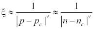
where v=0.88 is the correlation length critical exponent, p is probability that a channel can conduct the fluid, and pc denotes the critical probability related to percolation threshold [101].
HF- emissions 3.2.1.KHz band
A way to investigate transient phenomena is to analyze a sequence of distinct time windows of short duration into the detected pre-seismic time series. The aim is to discover a clear difference of dynamical characteristics as the catastrophic event is approaching. In order to develop a quantitative identification of kHz EM precursors, the concepts of entropy and tools from information theory are used in order to identify statistical patterns [4,12-31]. It is expected that a significant change of a statistical pattern represents a deviation from normal behavior, revealing the presence of an anomaly. Symbolic dynamics provide a rigorous way of looking at "real" dynamics. First, a symbolic analysis [4,22,23,26,28,102-104] of experimental data is attempted, in terms of Shannon n-block entropy, Shannon n-block entropy per letter, conditional entropy, entropy of the source and T-entropy. It is well-known that Shannon entropy works best in dealing with systems composed of subsystems, which can access all the available phase space and which are either independent or interact via short-range forces. However, a central property of the earthquake preparation process is the possible occurrence of coherent large-scale collective behavior with a very rich structure, resulting from repeated non-linear interactions among the constituents of the system. Consequently, non-extensive Tsallis entropy is an appropriate tool for investigating the launch of a kHz EM precursors [21,22,31,66]. It has been shown [4,16,19,22,55] that the techniques based on critical dynamics discriminate also clearly the recorded kHz EM anomalies from the background: they are characterized by a significantly lower complexity (or higher organization). The analysis with Approximate Entropy verified the results of symbolic dynamics [21,22,67]. On the other hand, the fractal spectral analysis [4,13,14,17,20,21,25,27-30,48,49,70,105] offers additional information concerning signal/noise discrimination mainly due to two facts. First, it shows that the candidate kHz precursor follows the fractional Brownian motion (fBm)-model while, on the contrary, the background follows the 1/f-noise model. Second, it implies that the candidate kHz precursor has persistent behavior [4,13,14,17,20,21]. The existence of persistency in the candidate precursor is confirmed by R/S analysis, while the conclusion that the anomaly follows the persistent fBm-model is verified by Detrended Fluctuation Analysis.
The abrupt simultaneous appearance of both high organization and persistency in a launched kHz anomaly implies that the underlying fracto-electromagnetic process is governed by a positive feedback mechanism [4,13,14,17,20,21,25,27-30]. Such a mechanism is consistent with the anomaly's being a candidate precursor. Of course, such an analysis cannot establish, independently, the precursory value of a certain anomaly. Much remains to be done to tackle precursors systematically. It is a difficult task to rebate two events separated in time, such as a candidate kHz EM precursor and the ensuing earthquake. It remains to be established whether different approaches could provide additional information that would allow one to accept the seismogenic origin of the recorded kHz EM anomalies and link these to a crucial stage of earthquake generation, i.e., the kHz EM anomalies are associated with the fracture of asperities that are distributed along the fault sustaining the system.
MHz band: It has been shown that the MHz EM precursors present strong anti-persistent behavior [4,10-26]. This behaviour indicates an underlying non-linear feedback of the system that "kicks" the crackopening rate away from extremes [20]. This anti-persistent behavior is similar to the one found in systems which undergo a continuous phase transition at equilibrium [4,16,19,22,55]. Heterogeneity could account for the appearance of a stationary-like behavior in the antipersistent part of the pre-fracture MHz EM time series. A published statistical method of analysis of critical fluctuations has shown that the detected precursory MHz anomalies, could be described in analogy to a continuous thermal phase transition. More specifically, it has been shown [4,16,19,22,55] that an underlying strong critical behavior is consistent to a criterion: the majority of trajectories in the properly defined laminar region carry out information about the underlying criticality. The MHz EM precursors follow this criterion.
A thermal second-order phase transition is associated with a "symmetry breaking" [4,16,19,22,55]. To gain insight into the catastrophic character of the fracture phenomena, the evolution of the "symmetry breaking" with time has been elucidated for nonequilibrium- irreversible processes. The analysis showed that the system is gradually driven out of equilibrium. Through this the time was estimated beyond which the process which generates the pre-seismic MHz EM emission could continue only as non-equilibrium instability. More precisely, the analysis revealed the following significant issues: (i) The critical epoch (critical window) during which the short-range correlations evolve to long-range, (ii) The epoch of the "symmetry breaking" occurrence, (iii) The integration of the "symmetry breaking". It is generally accepted that the terminal phase of the earthquake preparation process is accompanied by significant increase in localization and directionality. It is hence important to distinguish characteristic epochs in the evolution of precursory MHz EM activity and to link these to the equivalent last stages in the earthquake preparation process. Tracing of "symmetry-breaking" may signalize that the micro-fracture propagation has finished in the heterogeneous component of the focal area, which surrounds the backbone of the strong asperities on the fault plane: the rupture has been obstructed at the boundary of the backbone of strong asperities: The "siege" of asperities has already been started [20].
It is important to mention that MHz radiation precedes kHz both at the large (geophysical) and at the small (laboratory) scale [4,10-26]. Attention should be given to the fact that the time lags between the pre-earthquake EM anomalies and the impeding earthquakes are different among the MHz and the kHz precursors. This remarkable asynchronous emergence of the MHz and the kHz precursors indicates that they refer to different stages of the earthquake preparation process [4]. A significant issue for science is to attempt associations between the numerous detectable EM observations, that appear one after the other, to the consecutive processes within the Earth's crust [4,10-26].
It has been clarified that the emergence of a MHz EM anomaly is a necessary but not a sufficient condition for the earthquake occurrence [4,10-26]. Indeed, although numerous MHz EM anomalies have been detected with clear strong, critical and anti-persistent behavior, these were not combined with the occurrence of a significant earthquake. Noticeably is that any possible relations of these anomalies should be excluded if associated to magnetic storm activity, solar flare activity, or, man-made electromagnetic sources.
Conclusion
The present paper attempted a systematic review of electromagnetic precursors focusing on those of the ULF, LF and HF range. Several investigators have reported pre-seismic electromagnetic disturbances that were claimed to be precursory. The vast majority of the reported electromagnetic disturbances were analyzed visually. Advanced techniques based on Natural Time, Detrended Fluctuation Analysis and fractals have been reported for the ULF precursors. Numerous LF and HF pre-earth-quake electromagnetic disturbances have been analyzed through evolution of fractal dimension, Hurst exponent, DFA and several metrics of entropy. Either the analysis of long memory of the earthquake generating system or the compilation of the system's self-organization, have provided significant findings regarding the nodal evolution stages of certain earthquakes. Much research needs to be done so as to delineate the process of generation of earthquakes in terms of science.
References
- Keilis-Borok VI, Soloviev AA (2003) Nonlinear Dynamics of the Lithosphere and Earthquake Prediction. Springer, Heidelberg 348.
- Keilis-Borok V (2002)Earthquake Prediction: State-of-the-Art and Emerging Possibilities. Annu Review Earth and Pl Sc 30: 1-33.
- Hayakawa M, Hobara Y (2010) Current status of seismo-electromagnetics for short-term earthquake prediction. Geomatics, Nat Haz Risk 1:115-155.
- Eftaxias K (2010) Footprints of non-extensive Tsallis statistics, self-affinity and universality in the preparation of the L'Aquila earthquake hidden in a pre-seismic EM emission. Physica A 389: 133-140.
- Nikolopoulos D, Petraki E, Marousaki A, Potirakis S, Koulouras G, et al. (2012) Environmental monitoring of radon in soil during a very seismically active period occurred in South West Greece. J EnvironMonit 14: 564-578.
- Molchanov A, Kopytenko A, Voronov M, Kopytenko A, Matiashviali G, et al. (1992) Results of ULF magnetic field measurements near the epicenters of the Spitak (Ms= 6.9) and Loma-Prieta (Ms= 7.1) earthquakes: comparative analysis. Geophys Res Lett 19: 1495-1498.
- Aggarwal P, Sykes R, Simpson W, Richards G (1975) Spatial and temporal variations in ts/tp and in P wave residuals at Blue Mountain Lake, New York: Application to earthquake prediction. JGeophys Res 80:718-732.
- Cicerone R, Ebel J, Britton J (2009) A systematic compilation of earthquake precursors. Tectonophys 476: 371-396.
- Parvaiz K, Sharad T, Azad M, Purushottam B, Purohit P, et al. (2011) Scientific efforts in the direction of successful earthquake prediction.Int JGeomaticsGeosci 1: 669-677.
- Eftaxias K, Kapiris P, Polygiannakis J, Bogris N, Kopanas J, et al. (2001) Signature of pending earthquake from electromagnetic anomalies. Geophys Res Lett 29: 3321-3324.
- Hadjicontis V, Mavromatou C, Eftaxias K (2002) Preseismic earth’s field anomalies recorded at Lesvos station, north-eastern Aegean. ActaGeophysicaPolonica 50: 151-158.
- Eftaxias K, Kapiris P, Dologlou E, Kopanas J, Bogris N, et al. (2002) EM anomalies before the Kozani earthquake: a study of their behavior through laboratory experiments. Geophys ResLett 29: 69-1-69-4.
- Kapiris P, Polygiannakis J, Peratzakis A, Nomicos K, Eftaxias K (2002) VHF-electromagnetic evidence of the underlying pre-seismic critical stage. Earth Planets Space 54: 1237-1246.
- Kapiris P, Eftaxias K, Nomikos K, Polygiannakis J, Dologlou E, et al. (2003) Evolving towards a critical point: A possible electromagnetic way in which the critical regime is reached as the rupture approaches. Nonlinear Process Geophys 10: 511-524.
- Kapiris P, Eftaxias K, Chelidze T (2004) Electromagnetic Signature of Prefracture Criticality in Heterogeneous Media.Phys Rev Lett 92: 065702-1/065702-4.
- Contoyiannis Y, Kapiris P, Eftaxias K (2005) Monitoring of a preseismic phase from its electromagnetic precursors. Phys Rev E 71: 066123(1-14).
- Eftaxias K, Kapiris P, Balasis G, Peratzakis A, Karamanos K, et al. (2006) Unified approach to catastrophic events: from the normal state to geological or biological shock in terms of spectral fractal and nonlinear analysis. Nat Haz Earth Sys Sci 6: 205-228.
- Eftaxias K, Panin V, Deryugin Y (2007) Evolution-EM signals before earthquakes in terms of meso-mechanics and complexity. Tectonophys 431: 273-300.
- Contoyiannis Y, Eftaxias K (2008) Tsallis and Levy statistics in the preparation of an earthquake. Nonlinear ProcessGeophys 15: 379-388.
- Eftaxias K, Contoyiannis Y, Balasis G, Karamanos K, Kopanas J, et al. (2008) Evidence of fractional-Brownian-motion-type asperity model for earthquake generation in candidate pre-seismic electromagnetic emissions. Nat Haz Earth Sys Sci 8: 657-669.
- Eftaxias K, Athanasopoulou L, Balasis G, Kalimeri M, Nikolopoulos S, et al. (2009) Unfolding the procedure of characterizing recorded ultra low frequency, kHz and MHz electromagnetic anomalies prior to the L’Aquila earthquake as pre-seismic ones - Part 1. Nat Haz Earth Sys Sci9: 1953-1971.
- Eftaxias K, Balasis G, Contoyiannis Y, Papadimitriou C, Kalimeri M, et al.(2010) Unfolding the procedure of characterizing recorded ultra low frequency, kHZ and MHz electromagnetic anomalies prior to the L’Aquila earthquake as pre-seismic ones - Part 2. NatHaz Earth Sys Sci 10: 275-294.
- Minadakis G, Potirakis S, Nomicos C, Eftaxias K (2012) Linking electromagnetic precursors with earthquake dynamics: An approach based on non-extensive fragment and self-affine asperity models. Physica A 391: 2232-2244.
- Potirakis S, Minadakis G, Eftaxias K (2012) Analysis of electromagnetic pre-seismic emissions using Fisher information and Tsallis entropy. Physica A 391: 300-306.
- Balasis G, Mandea M (2007) Can electromagnetic disturbances related to the recent great earthquakes be detected by satellite magnetometers? Tectonophys 431: 173-195.
- Balasis G, Daglis I, Papadimitriou C, Kalimeri M, Anastasiadis A, et al. (2008) Dynamical complexity in Dst time series using non-extensive Tsallis entropy. Geophys Res Lett 35: L14102 (1-6).
- Petraki E, Nikolopoulos D, Fotopoulos A, Panagiotaras D, Koulouras G, et al. (2013) Self-organised critical features in soil radon and MHz electromagnetic disturbances: Results from environmental monitoring in Greece. ApplRadiat Is 72: 39-53.
- Petraki E, Nikolopoulos D, Fotopoulos A, Panagiotaras D, Nomicos C, et al. (2013) Long-range memory patterns in variations of environmental radon in soil. Anal Method 5: 4010-4020.
- Nikolopoulos D, Petraki E, Vogiannis E, Chaldeos Y, Giannakopoulos P, et al. (2014) Traces of self-organisation and long-range memory in variations of environmental radon in soil: Comparative results from monitoring in Lesvos Island and Ileia (Greece). JRadioanal Nuclear Chem 299: 203-219.
- Petraki E, Nikolopoulos D, Chaldeos Y, Coulouras G, Nomicos C, et al. (2014) Fractal evolution of MHz electromagnetic signals prior to earthquakes: results collected in Greece during 2009.Geomatics, NatHazRisk (in press).
- Kalimeri M, Papadimitriou C, Balasis G, Eftaxias K (2008) Dynamical complexity detection in pre-seismic emissions using non-additive Tsallis entropy.Physica A 387: 1161-1172.
- Varotsos P, Sarlis N, Skordas E (2011) Scale-specific order parameter fluctuations of seismicity in natural time before main shocks.EPL (Europhysics Letters) 96: 59002-p1/59002-p6.
- Sarlis N, Skordas E, Varotsos P, Nagao T, Kamogawa M, et al. (2013) Minimum of the order parameter fluctuations of seismicity before major earthquakes in Japan. Proc National Acad U S Am 110: 13734-13738.
- Warwick J, Stoker C, Meyer T (1982) Radio Emission Associated With Rock Fracture: Possible Application to the Great Chilean Earthquake of May 22, 1960. J Geophys Res 87: 2851-2859.
- Smith B, Johnston M (1976) Atectonomagnetic effect observed before a magnitude 5.2 earthquake near Hollister, California. J Geophys Res 81: 3556-3560.
- ZhaoY, Qian F (1994) Geoelectric precursors to strong earthquakes in China. Tectonophys 233: 99-113.
- Wallace R, Teng T (1980) Prediction of the Sungpan-Pingwu earthquakes, 1976. Bull SeismolSoc Am 70: 1199-1223.
- Gokhberg M, Morgounov V, Yoshino T, Tomizawa I (1982) Experimental Measurement of Electromagnetic Emissions Possibly Related to Earthquakes in Japan. J Geophys Res 87: 7824-7828.
- Gershenzon N, Gokhberg M (1993) On the origin of electrotelluric disturbances prior to an earthquake inKalamata, Greece. Tectonophys 224: 169-174.
- Kopytenko Y, Matiashviali T, Voronov P, Kopytenko E, Molchanov O (1993) Detection of ultra-low-frequency emissions connected with the Spitak earthquake and its aftershock activity, based on geomagnetic pulsations data at Dusheti and Vardzia observatories. Phys Earth Planet In 77: 85-95.
- Fraser-Smith A , Bernardi A, McGill P, Ladd M, Helliwell R, Viilard O (1990) Low-frequency magnetic field measurements near the epicenter of the Ms 7.1 Loma Prieta earthquake.Geophys Res Lett 17: 1465-1468.
- Serebryakova O, Bilichenko S, Chmyrev V, Parrot M, Rauch J, et al. (1992) Electromagnetic ELF radiation from earthquake regions as observed by low-attitude satellites. Geophys Res Lett19: 91-94.
- Dea J, Hansen P, Boerner W (1993) Long-term EMF background noise measurements, the existence of window regions and applications to earthquake precursor emission studies. Phys Earth PlanetIn 77: 109-125.
- Shalimov S, Gokhberg M (1998) Lithosphere-ionosphere coupling mechanism and its application to the earthquake in Iran on June 20, 1990.A review of ionospheric measurements and basic assumptions. Phys Earth Planet In 105: 211-218.
- Ondoh T (1998) Ionospheric disturbances associated with great earthquake of Hokkaido southwest coast, Japan of July 12, 1993. Phys Earth Planet In 105: 261-269.
- Hayakawa M, Kawate R, Molchanov O, Yumoto K (1996) Results of ultra-low-frequency magnetic field measurements during the Guam earthquake of 8 August 1993.Geophys Res Lett 23: 241-244.
- Hayakawa M, Ito T (1999) Fractal analysis of ULF geomagnetic data associated with the Guam earthquake on August 8, 1993. Geophys Res Lett26: 2797-2800.
- Smirnova, N, Hayakawa M (2007) Fractal characteristics of the ground-observed ULF emissions in relation to geomagnetic and seismic activities. JAtmos Solar-Terrestrial Phys 69: 1833-1841.
- Hayakawa M, Ida Y, Gotoh K (2005) Multifractal analysis for the ULF geomagnetic data during the Guam earthquake. Electromagnetic Compatibility and Electromagnetic Ecology, 2005.Proc IEEE 6thInt Symposium on 21-24 June 2005:239 - 243.
- Fujinawa Y, Takahashi K (1998) Electromagnetic radiations associated with major earthquakes. Phys Earth Planet In 105: 249-259.
- Enomoto Y, Tsutsumi A, Fujinawa Y, Kasahara M, Hashimoto H (1997) Candidate precursors: pulse-like geoelectric signals possibly related to recent seismic activity in Japan. Geophys J Int 131: 485-494.
- Maeda K, Tokimasa N (1996) Decametric radiation at the time of the Hyogo-ken Nanbu earthquake near Kobe in 1995. Geophys Res Lett23: 2433-2436.
- Bernard P, Pinettes P, Hatzidimitriou P, Scordilis E, Veis G, et al. (1997) From precursors to prediction: a few recent cases from Greece. Geophys J Int 131: 467-477.
- Contoyiannis Y, Diakonos F., Kapiris P, Peratzakis A, Eftaxias K (2004) Intermittent dynamics of critical pre-seismic electromagnetic fluctuations. PhysChem Earth 29:397-408.
- Varotsos P, Sarlis N, Eftaxias K, Lazaridou M, Bogris N, et al. (1999) Prediction of the 6.6 Grevena-Kozani Earthquake of May 13, 1995. PhysChem Earth 24: 115-121.
- Varotsos P, Sarlis N, Skordas E (2003) Electric Fields that “Arrive” before the Time Derivative of the Magnetic Field prior to Major Earthquakes. Phys Rev Lett 91:148501-1/148501-4.
- Varotsos P, Sarlis N, Skordas E, Lazaridou M (2007) Electric pulses some minutes before earthquake occurrences. ApplPhysLett 90: 064104-1/064104-3.
- Hayakawa M, Ohta K, Maekawa S, Yamauchi T, Ida Y, et al. (2006) Electromagnetic precursors to the 2004 Mid Niigata Prefecture earthquake. PhysChem Earth 31: 351-364.
- Yonaiguchi N, Ida Y, Hayakawa M, Masuda S (2007) Fractal analysis for VHF electromagnetic noises and the identification of preseismic signature of an earthquake. J Atmos Solar-Terrestrial Phys 69: 1825-1832.
- Biagi P, Ermini A, Kingsley S (2001) Disturbances in LF Radio Signals and the Umbria-Marche (Italy) Seismic Sequence in 1997-1998. PhysChem Earth 26: 755-759.
- Karakelian D, Klemperer S, Fraser-Smith A, Thompson G (2002) Ultra-low frequency electromagnetic measurements associated with the 1998 Mw 5.1 San Juan Bautista, California earthquake and implications for mechanisms of electromagnetic earthquake precursors. Tectonophys 359:65-79.
- Nikolopoulos S, Kapiris P, Karamanos K, Eftaxias K (2004) A unified approach of catastrophic events. Nat HazEarth Sys Sci 4: 615-631.
- Kapiris P, Nomicos K, Antonopoulos G, Polygiannakis J, Karamanos K, et al. (2005) Distinguished seismological and electromagnetic features of the impending global failure: Did the 7/9/1999 M5.9 Athens earthquake come with a warning? Earth Planets Space 57: 215-230.
- Karamanos K, Peratzakis A, Kapiris P, Nikolopoulos S, Kopanas J, et al. (2005) Extracting preseismicelectromagnetic signatures in terms of symbolic dynamics. Nonlinear Process Geophys 12: 835-848.
- Potirakis S, Minadakis G, Nomicos C, Eftaxias K (2011) A multidisciplinary analysis for traces of the last state of earthquake generation in preseismic electromagnetic emissions. NatHaz Earth Sys Sci11: 2859-2879.
- Potirakis S, Minadakis G, Eftaxias K (2013) Relation between seismicity and pre-earthquake electromagnetic emissions in terms of energy, information and entropy content. Nat Haz Earth Sys Sci12: 1179-1183.
- Chuo Y, Liu J, Pulinets S, Chen Y (2002) Theionospheric perturbations prior to the Chi-Chi and Chia-Yi earthquakes. J Geodyn 33: 509-517.
- Ruzhin Y, Nomicos C (2007) Radio VHF precursors of earthquakes. Nat Haz 40: 573-583.
- Gotoh K, Hayakawa M, Smirnova N, Hattori K (2004) Fractal analysis of seismogenic ULF emissions. PhysChem Earth29: 419-424.
- Smirnova N, Hayakawa M, Gotoh K (2004) Precursory behavior of fractal characteristics of the ULF electromagnetic fields in seismic active zones before strong earthquakes. PhysChem Earth29: 445-451.
- Saroso S, Hattori K, Ishikawa H, Ida Y, Shirogane R, et al. (2009) ULF geomagnetic anomalous changes possibly associated with 2004-2005 Sumatra earthquakes. PhysChem Earth34:343-349.
- Parrot M (1994) Statistical study of ELF/VLF emissions recorded by a low-altitude satellite during seismicevents. J Geophys Res 99: 23339-23347.
- Yoshino T, Tomizawa I, Sugimoto T (1992) Results of statistical analysis of low-frequency seismogenic EM emissions as precursors to earthquakes and volcanic eruptions. Phys Earth Planet In 77:21-31.
- Varotsos P, Alexopoulos K (1984) Physical properties of the variations of the electric field of the earth preceding earthquakes, I. Tectonophys 110: 73-98.
- Varotsos P, Alexopoulos K (1984) Physical properties of the variations of the electric field of the earth preceding earthquakes, II, determination of epicenter and magnitude. Tectonophys 110:99-125.
- Bella F, Biagi P, Caputo M, Cozzi E, Della Monica G, et al. (1998) Field strength variations of LF radio waves prior to earthquakes in central Italy. Phys Earth Planet In 105:279-286.
- Vallianatos F, Nomikos K (1998) Seismogenic Radio-emissions as Earthquake Precursors in Greece. PhysChem Earth23:953-957.
- Yépez, E, Angulo-Brown, F, Peralta, JA, Pavía CG, González-Santos G (1995) Electric field patterns as seismic precursors. Geophys Res Lett22:3087-3090.
- Liu JY, Chen YI, Pulinets SA, Tsai YB, Chuo YJ (2000) Seismo-ionospheric signatures prior to M>6.0 Taiwan earthquakes. Geophys Res Lett27:3113-3116.
- Enescu BD, Enescu D, Constantin AP (1999) The use of electromagnetic data for short-term prediction of Vrancea (Romania) earthquakes: Preliminary data. Earth Planets Space 51: 1099-1117.
- Stavrakas I, Clarke M, Koulouras G, Stavrakakis G, Nomicos C (2007) Study of directivity ef-fect on electromagnetic emissions in the HF band as earthquake precursors: Preliminary results on field observations. Tectonophys 431: 263-271.
- Fujiwara H, Kamogawa M, Ikeda M., Liu JY, Sakata H, et al. (2004) Atmospheric anomalies observed during earthquake occurrences.Geophys Res Lett31: 1-4.
- Varotsos PA (2006) Recent Seismic Electric Signals (SES) activities in Greece. ActaGeophysica 54:158-164.
- Moore GW (1964) Magnetic disturbances preceding the 1964 Alaska earthquake. Nature 203:508-509.
- Shrivastava A (2014) Are pre-seismic ULF electromagnetic emissions considered as a reliable diagnostics for earthquake prediction? CurrSci 107: 596-60.
- Uyeda S (2000) In defense of VAN’s earthquake predictions, Eos, Transactions.AmGeophys Union 81:3-6.
- Uyeda S, Nagao T., Kamogawa M (2009) Short-term earthquake prediction: current status of seismo-electromagnetics. Tectonophys 470:205-213.
- P. Varotsos and M. Lazaridou (1991) Latest aspects of earthquake prediction in Greece based on Seismic Electric Signals. Tectonophys 188: 321-347.
- Varotsos P, Sarlis N, Lazaridou M, Bogris N (1996) Statistical evaluation of earthquake prediction results.Comments on the success rate and alarm rate.ActaGeophysicaPolonica 44: 329-347.
- Varotsos P, Alexopoulos K, Lazaridou M (1993) Latest aspects of earthquake prediction in Greece based on Seismic Electric Signals II. Tectonophys 224:1-37.
- Draganov AB, Inan US, Taranenko Yu N (1991) ULF magnetic signatures at the Earth's surface due to ground water flow: a possible precursor to earthquakes. Geophys Res Lett18:1127-1130.
- Sasai Y (1991) Tectonomagnetic modeling on the basis of the linear piezomagnetic effect. Bull Earthquake ResInstUniv Tokyo 66:585-722.
- Fitterman DV (1978) Electrokinetic and magnetic anomalies associated with dilatant regions in a layeredEarth. J Geophys Res 83:5923-5928.
- Fitterman DV (1979) Theory of electrokinetic-magnetic anomalies in a faulted half-space. J Geophys Res 84: 6031-6040.
- Varotsos P, Alexopoulos K, Nomicos K, Lazaridou M (1986) Earthquake prediction and electric signals. Nature 322:120.
- Dobrovolsky IP, Zubkov SI, Miachkin VI (1979) Estimation of the Size of Earthquake Preparation Zones. Pure ApplGeophys 117:1025-1044.
- Mizutani H, Ishido T (1976) A new interpretation of magnetic field variation associated with the Matsushiro earthquakes. JGeomagnGeoelectricity 28:179-188.
- Jouniaux L, Pozzi JP (1995) Streaming potential and permeability of saturated sandstones under triaxial stress: - consequences for electrotelluric anomalies prior to earthquakes. J Geophys Res 100:10197-10209.
- Surkov V, Uyeda S, Tanaka H, Hayakawa M (2002) Fractal properties of medium and seismoelectric phenomena. JGeodyn 33:477-487.
- Nicolis G, Gaspard P (1994) Toward a probabilistic approach to complex systems.Chaos, SolitonsFractals 4:41-57.
- Karamanos K, Nicolis G (1999) Symbolic dynamics and entropy analysis of Feigenbaum limit sets. Chaos, Solitons and Fractals 10:1135-1150.
- Karamanos K (2001) Entropy analysis of substitutive sequences revisited. J Physics A: MathGen 34: 9231-9241.
- Karamanos K, Dakopoulos D, Aloupis K, Peratzakis A, Athanasopoulou L, et al. (2006) Preseismic electromagnetic signals in terms of complexity. Phys Rev E 74:016104/1-016104/21.
- Smirnova N, Hayakawa M (2007) Fractal characteristics of the ground-observed ULF emissions in relation to geomagnetic and seismic activities. J Atmos Sola r-Terrestrial Phys 69:1833-1841.
Citation: Petraki E, Nikolopoulos D, Nomicos C, Stonham J, Cantzos D, et al. (2015) Electromagnetic Pre-earthquake Precursors: Mechanisms, Data and Models-A Review. J Earth Sci Clim Change 6: 250. Doi: 10.4172/2157-7617.1000250
Copyright: © 2015 Petraki E, et al. This is an open-access article distributed under the terms of the Creative Commons Attribution License, which permits unrestricted use, distribution, and reproduction in any medium, provided the original author and source are credited.
Share This Article
Open Access Journals
Article Tools
Article Usage
- Total views: 20440
- [From(publication date): 1-2015 - Apr 25, 2024]
- Breakdown by view type
- HTML page views: 15570
- PDF downloads: 4870