| Research Article |
Open Access |
|
| G H Erjaee1*, M Shahbazi1 and A Erjaee2 |
| 1Mathematics Department, Shiraz University, Shiraz, Iran |
| 2Assistant Professor, Pediatric Department, Shiraz University, Medical School, Shiraz, Iran |
| *Corresponding authors: |
G. H. Erjaee
Mathematics Department
Shiraz University
Shiraz, Iran
E-mail: erjaee@shirazu.ac.ir |
|
| |
| Received August 21, 2011; Published October 01, 2012 |
| |
| Citation: Erjaee GH, Shahbazi M, Erjaee A (2012) Dynamical Analysis of Mathematical Model Presented by Fractional Differential Equations, Describing the Interaction Between Leukemic Cancer Cells, T Cells and Drug Treatment with a Drug Optimal Control. 1:390. doi:10.4172/scientificreports.390 |
| |
| Copyright: © 2012 Erjaee GH, et al. This is an open-access article distributed under the terms of the Creative Commons Attribution License, which permits unrestricted use, distribution, and reproduction in any medium, provided the original author and source are credited. |
| |
| Abstract |
| |
| Obviously, one's primary motivation in producing any mathematical model is to describe a natural or artificial phenomenon by means of a model equation whose behavior is as close as possible to that of the original phenomenon. But this is often difficult, particularly when we are dealing with nonlinear behavior in natural complex phenomena such as the interaction between variety of cancers and immune cells. Thus, the choice of modeling schemes that produce models whose dynamics resembles those of their physical counterparts is a major challenge in mathematical molding. Ordinary differential equations and partial differential equations are just some of the mathematical tools that are been used in deriving these mathematical models. In this article, we have used fractional differential equations for our derivation. In this derivation, a mathematical model describes the growth or terminates myelogenous leukemia blood cancer’s cells against naive T-cell and effective T-cell cells of body. Using this model, we have studied the dynamic behavior describing the transaction between bodies' effective T cell, naive T cell and chronic myelogenous leukemia in one side and drug in other side. The most important feature of equations with fractional order derivatives is their non-localization. We expect that our fractional differential equations model will be superior to its ordinary differential equations counterpart in facilitating understanding of the natural immune interactions to tumor and of the detrimental side-effects which chemotherapy may have on a patient’s immune system. Using this system, we will study the optimized drug dose in chronic myelogenous leukemia treatment with two methods namely targeted therapy and broad cytotoxic therapy. |
| |
| Keywords |
| |
| Non-linear dynamics; Fractional differential equations; Cancer chemotherapy; Optimal drug control |
| |
| Mathematical Subject Classification |
| |
| 37N25, 37N35 and 44A55. |
| |
| Introduction |
| |
| Drug therapy is a way to cure cancer. It is clear that, the drug dose is important for cancer specialists. Considering the weakness of immunology system in cancer affected patients, drug overdose may results in additional problems for their body. |
| |
| Chronic myelogenous leukemia (CML) is a kind of blood cancer and occurs in adults about 15 percent [1]. The age average for blood cancer patients ranges between 45-55 years old. The occurrence rate is one or three among per 100000 individuals [1]. In most CML types, leukemic cells are divided to an unmoral Chromosome which can't be found neither in non-blood white cells nor in any of body’s cells [2]. Consequently, a displacement will be occurred between Chromosome 9 and 22 in such a way that Chromosome 9 will be longer than normal state and Chromosome 22 will be short which is called Chromosome Philadelphia (Ph) [2]. This Chromosome produce an unmoral protein namely Tyrosine kinase (Ber-Abl). This change results in conversion of bone marrow cells to abnormal leukemic cells [3,4]. Structural knowledge of Ber-Abl has led to the development of a drug, imatinib mesylate (known as Gleevec in the U.S. and henceforth referred to as imatinib), that blocks the abnormal protein, thus removing the proliferative advantage that it provides to cancer cells. Imatinib is highly specific to binding with Ber-Abl, and hence, generally has mild side effects [2]. One of the obtained successes in this regard was related to Food and Drug Administration (FDA) for detecting CML diseases in December, 2002 [5]. Bone marrow transplantation is a curative treatment option for some patients, but transplant-related mortality rates can be above 40 percent [6]. Prior to the development of imatinib, treatments such as hydroxyuea, cytarabine, interferonalfa or combination of them were used to treat CML [5]. The action of these therapies is against broad classes of cells, and so treatment usually results in severe side effects. Several studies suggest that combination of imatinib with a broader chemotherapy has the potential to perform better than imatinib alone [7-10]. |
| |
| Recently, the models used for analyzing the cancer reaction against drug therapy could assist physicians in cancer treatment. Therefore, using optimized control methods which minimized damages to body can play an important role in cancer treatment. In this field, researchers such as Fokas et al. [11] and Adimy et al. [12] have presented CML models in 1991 and 2005, respectively. A mathematical model has also presented by Afenya and Bentil in 1998 [13] for blood cancer. Periodic mathematical models for CML have presented by Mackey and Menjouet in 2004. |
| |
| In this article, the ordinary differential equation (ODE) which is presented by Moore and Li for brain blood cancer [14] is re-derived using fractional differential equation (FDE). We claim that our FDE model will be superior to its ODE counterpart in facilitating understanding of the natural immune interactions to tumor and of the detrimental side effects which chemotherapy may have on a patient’s immune system. Summarizing the advantages of our FDE model over previous ones, first as Andrew Einstein described in his research [15] at Mount Sinai School of Medicine, some cells in various body organs have a rugged surface that cannot be properly understand using ordinary calculus, but it may be amenable to studies using fractional calculus. In addition, since differentiability is not required in accordance with the definition of FDE with order between 0 and 1, so these equations can be used in non-smooth domains. Furthermore, whereas in the definition of the classical derivative of a function at a point we use just two points in the neighborhood of that point in the definition of the fractional derivative we use all the points in a neighborhood of the point. Obviously, by using all of the information available in these points we obtain more accurate results in subsequent applications. The last property that is so-called non-local property will closely reflect reality and is a primary reason why FDE are increasingly applied to dynamical systems. |
| |
| Therefore, in this article, first we will introduce a FDE model to present the interaction between naive T cells, effectors T cells, and CML cancer cells in cancer dormancy. Then, we will discuss the dynamical behavior of this model by identifying the fixed points and determining their stability characteristics. To find the solutions of this FDE system, we will discretize the system by using Grunwald- Letnikov discretization method [16,17] then, we will find the results by using software tools such as MATLAB™. In this FDE model, by adding chemotherapy drug concentration to the interaction between naive T cells, effectors T cells, and CML cancer cells and considering the same three cells populations as in the first FDE, we will have our second model in the form of FDE. Now, similar to the way in which have been done in classical ODE systems, we will discuss the dynamic behavior of the first system and determine the stability type of the various feasible fixed points. One of the main goals in using fractional order instead of classical integer order derivative in our model is to obtain more accurate results in chemotherapy optimal control. For this optimality, similar to the targeted therapy (such as imatinib) and broad cytotoxic therapy (such as cytarabine) methods used by Moore and Li [14], we will use the processors in our FDE model. Obviously, in the processing of this optimality we need to solve our FDE system numerically. To facilitate this solution, as in above first FDE system, we will apply Grunwald-Letnikov method to discretize the model and then, use MATLAB™ software to find the results. |
| |
| As we stated before, we will expect more accurate results in solving our FDE systems as compared to the results found by classical ODE methods. |
| |
| Dynamical Analyses of Tumor without Treatment in the FDE Model |
| |
| The first model that we consider here is a three cells population model describing the interaction between the cancer cell population (C), the naive T cell population (Tn) and effector T cell population (Te). We assume that the effector T cells are specific to CML, activated by the presence of CML antigen. If we suppose these three cells evolve with independent variable time, then we can present our model in the form of FDE as follows. |
| |
 , , |
| |
 , , |
| |
 |
| |
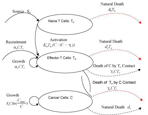
| This model is similar to the classical ODE model presented by Seema Nanda and Helen Moore [14]. Here, we use the same order derivatives α∈(0,1) for all three equations, where Tn(0), Te (0) and C(0) are known initial values. All of the parameter values in the above equations are assumed to be positive. The structure of the equations guarantees non-negative solutions for the state variables, (t), (t) and C(t) [2]. The negative terms in the above equations represent losses from the cell populations while the positive terms are source terms for the cell populations (Figure 1). The last term in the first equation (which has a Michaelis–Menten factor) represents the decline in Tn cells due to encounters with CML antigen in the lymph nodes. As the population of Tn cells is very small in comparison to the CML cells, this term takes into account the saturation effect of CML cells in the lymph nodes. Since some of these lost Tn cells reappear as effector T cells (Te), a Michaelis-Menten factor also shows up in the first term in Eq. (2). The model assumes Gompertz growth for CML cells as indicated by the growth term in Eq. (3). Also, it is assumed that encounters in the blood between Te cells and C cells are modeled by the law of mass action, i.e., the effect of these cells on each other is based on the sizes of the two cell populations, and there is no saturating effect in the blood circulation system. The lower case parameters (Sn, an, etc.) in the above equations are all constants, as is Cmax [2]. |
| |
|
|
Figure 1: Cell population diagram. In this figure, solid curves with arrows represent source terms (such as proliferation and activation), dotted curves without arrows represent interaction terms (such as contact between cells), and dashed curves with arrows represent loss of cells (such as death). Curves with arrows signify movement into or out of a population, while curves without arrows only signify interactions between populations [14]. |
|
| |
| Here, we use the same values for the parameters as in [14] and appear in table 1. |
| |
|
|
Table 1: Parameter Values. |
|
| |
| As with ODE, the dynamic status of system (1-3) can be studied. First, we should find the fixed points of system (1-3) and then their stability should be analyzed. In system (1-3) we reach the problem parameters to 8 using standard rescaling (non-dimensionalization) [ 14]. Tn is rescaled with factor dn/Sn, Te is rescaled with factor γc/dn, and C is rescaled with factor γe/dn and t is rescaled with factor dn. With these rescaling system (1-3) yields |
| |
 , , |
| |
 , , |
| |
 . . |
| |
Where the new factors are defined as  , , , , , , , , , , . . |
| |
| For finding the fixed points considering to C=0 (no cancer cell), Eq. (4) implies that Tn=1 and Eq. (5) implies that Te=0. There are no any other fixed points for C=0. So, we have just P1= (1, 0, 0). To find the other fixed points, for the case C≠0, from Eqs. 4-6 we have |
| |
 |
| |
The third term on the right-hand side of Eq. (7) is logarithmic in C and hence, increases as C increases. For the factors of the fourth term to be zero, C must be negative (for the clinically feasible ranges of parameters in table 1). Thus, this fourth term is a rational function which decreases as C increases (when C is positive), and so there is at most one value of C on which makes the right-hand side of Eq. (7) to be zero. Therefore, the second fixed point will be  and for this we need and for this we need |
| |
 |
| |
| Note that again, for biological purpose the populations of Tn, Te and C should not be negative. Therefore, we have at most one real fixed point, rather than P1 for this system. |
| |
To determine the stability analysis of the cell populations near the fixed points, according to the Matignon theorem [18], the fixed points of FDE system (4-5) is asymptotically stable if and only if the eigen values of related linearized system satisfied in  . However, since the minimum value of α ∈ (0,1) that we chose here is closed to one, namely α = 95.0, the stability domain for the eigen values of the linearized system will be (almost) left hand side of R2 coordinates, i.e. the place that the real part of eigen values are negative. This means that we may use the same theorems as in ODE systems for the stability analysis of our FDE system. . However, since the minimum value of α ∈ (0,1) that we chose here is closed to one, namely α = 95.0, the stability domain for the eigen values of the linearized system will be (almost) left hand side of R2 coordinates, i.e. the place that the real part of eigen values are negative. This means that we may use the same theorems as in ODE systems for the stability analysis of our FDE system. |
| |
| Therefore, for the stability analysis of the fixed points, we need to determine the linearization of the system (4-6). This linearization yields |
| |
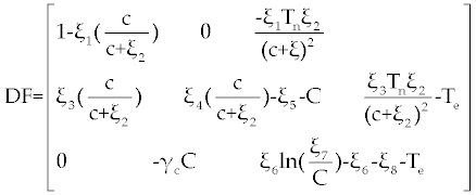 |
| |
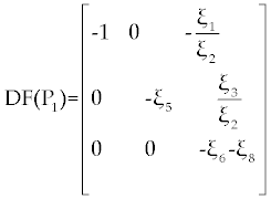
| By substituting P 1= (1, 0, 0) in this matrix we get |
| |
 |
| |
By easy calculation, the eigen values of this Jacobian matrix will be λ1= −1, λ2= −ξ5 and λ3= −ξ6 − ξ8. It is clear that λ1, λ2 and λ3 all have negative (real) sign Therefore, P1 is stable. For the second fixed point  (if exists), we may use a similar analysis as above. However, due to the long and complicated calculations, such as the one has done by Routh test [19], presents a kind of non-algebraic system that cannot be solved analytically [13]. (if exists), we may use a similar analysis as above. However, due to the long and complicated calculations, such as the one has done by Routh test [19], presents a kind of non-algebraic system that cannot be solved analytically [13]. |
| |
As an alternative, we can calculate the eigen values for a wide variety of possible parameter values, as has done in [14], by systematically sampling through the ranges listed in table 1. Using this method to find the eigen values of the matrix (8), we may use different sampling intervals for  and and  . For example, using the interval (0, 5000) for populations , . For example, using the interval (0, 5000) for populations ,  and (1, 400000) for and (1, 400000) for  all of the eigen values were either negative real or were imaginary with all of the real parts bounded above by -1.000076. The large ranges of all of the eigen values were either negative real or were imaginary with all of the real parts bounded above by -1.000076. The large ranges of  and and  used to calculate the eigen values give reasonable confidence that the eigen values have negative real parts for this fixed point. Hence, we assume the second fixed point to be asymptotically stable. used to calculate the eigen values give reasonable confidence that the eigen values have negative real parts for this fixed point. Hence, we assume the second fixed point to be asymptotically stable. |
| |
| Discretization and Numerical Solution in Fractional Mode |
| |
As we discussed above, linear stability analysis of system (1-3) or (4-6), around its fixed points, were similar to that of its ODE counterpart. However, to solve FDE system (1-3) first we need to discretize it. Among the several discretization methods that are available for the fractional derivative  , we used the one that have generated by Grunwald- Letnikov [16,17]. In this method , we used the one that have generated by Grunwald- Letnikov [16,17]. In this method  is approximated by is approximated by |
| |
 , , |
| |
where, l is the step size and [t] is the integer part of t. Using this method for system (1-3),  is replaced by is replaced by |
| |
| |
 |
| |
where tn = nl and  is Grunwald-Letnikov coefficients defined by is Grunwald-Letnikov coefficients defined by |
| |
 |
| |
We may calculate  with the following recursive formula too. with the following recursive formula too. |
| |
 |
| |
| Now, Using Eq.9, system (1-3) discretize as follows. |
| |
 , , |
| |
 , , |
| |
 . . |
| |
| By simple calculations, system (11-13) yields the following recursive formulas. |
| |
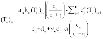 , , |
| |
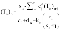 , , |
| |
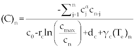 . . |
| |
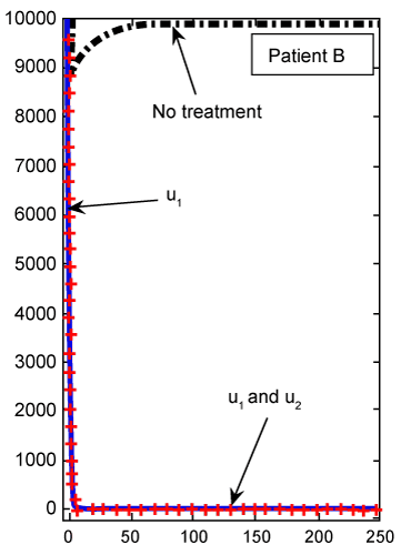
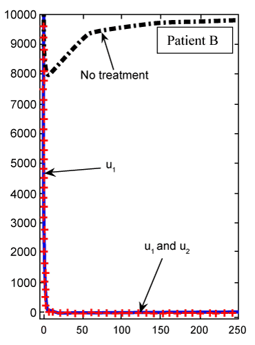
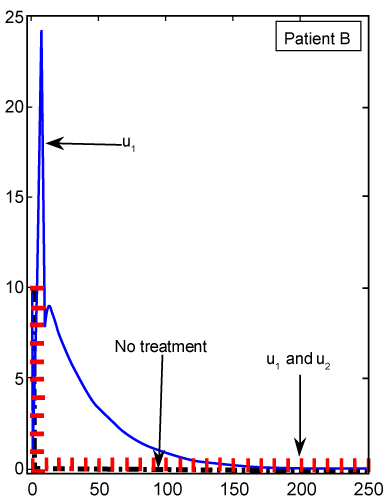
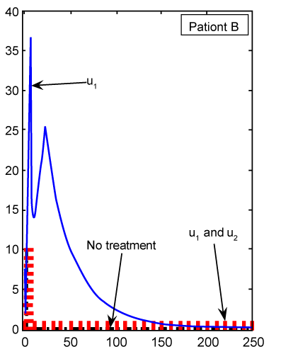
| The numerical results carried out by using MATLAB™ software for two sets of parameters given in table 1 (patients A and B) with initial values (Tn)0=1510, (Te)0=10 and C0=10000. These results illustrated in figures 2- 9 for both patients, whom we label A and B for different values of derivative order α. Each set of parameters defines an individual (hypothetical) patient for whom we determine an optimal dosing strategy. As we can see in figures 2- 5, the graphs shown by dashpoints (black color) present tumor concentration, C, for patients A and B with derivative orders α=1 and α=0.95. If we look at these graphs more precisely, we claim that the ones belong to the fractional order derivatives (α=0.95) behaves more naturally than the one belong to classical order (α=1). For example, comparing the C carves in figures 4 and 5, the one belong to classical order goes from initial value 10000 to the minimum point 8500 (Figure 4). While, the one belong to the fractional order goes to the minimum point 8000 and then growth up by a natural slop. It seems that the model with fractional order is closer to the nature of the body defense system. However, this claim should be verified by more precise clinical data. |
| |
|
|
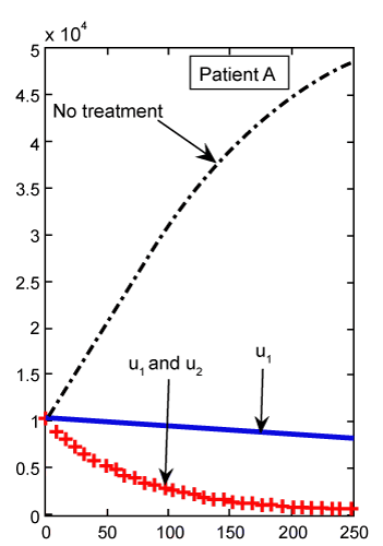
Figure 2: Numerical results for cancer cell population (C) (patient A) found from ODE system for classical derivative order α=1. |
|
| |
|
|
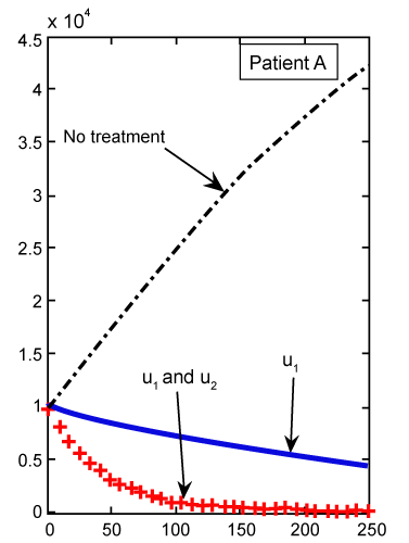
Figure 3: Numerical results for cancer cell population (C) (patient A) found from FDE system for fractional derivative order α=0.95. |
|
| |
|
|
Figure 4: Numerical results for cancer cell population (C) (patient B) found from ODE system for classical derivative order α=1. |
|
| |
|
|
Figure 5: Numerical results for cancer cell population (C) (patient B) found from FDE system for fractional derivative order α=0.95. |
|
| |
|
|
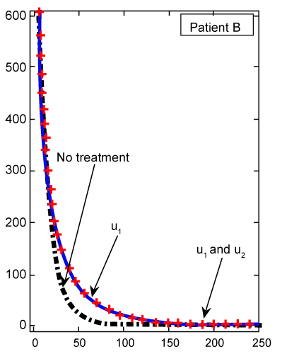
Figure 6: Numerical results for naive T cell population (Tn) (patient B) found from ODE system for classical derivative order α=1. |
|
| |
|
|
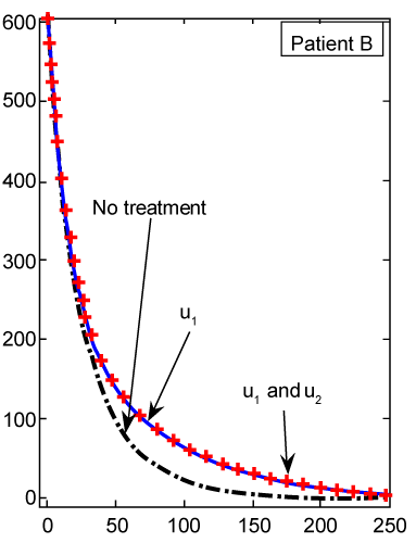
Figure 7: Numerical results for naive T cell population (Tn) (patient B) found from FDE system for fractional derivative order α=0.95. |
|
| |
|
|
Figure 8: Numerical results for effector T cell population (Te) (patient B) found from ODE system for classical derivative order α=1. |
|
| |
|
|
Figure 9: Numerical results for effector T cell population (Te) (patient B) found from FDE system for fractional derivative order α=0.95. |
|
| |
| FDE Model with Drug Treatment |
| |
| In this section, the ODE model presented by Moore and Li for brain blood cancer [14] is derived using FDE. So, if we consider the same system (1-3) with three cells populations along with a chemotherapy treatment describing the growth, death, and interactions of each cells, then such this system can be formulated by the means of FDE as follows. |
| |
 , , |
| |
 , , |
| |
 . . |
| |
| In this system (0), (0) and C(0) are known initial values and time dependent drug efficacies are incorporated using u1(t) and u2(t). Setting u 1(t) ≡ 0 and u2(t) ≡ 1 in the Eqs. (17-19) would give the same model described for the dynamics of the disease without treatment. All of the parameter values in these equations are assumed to be positive. Again, the structure of the equations guarantees non negative solutions for the state variables, (t), (t) and C(t). The negative terms in the above equations represent losses from the cell populations while the positive terms are source terms for the cell populations [2]. |
| |
| The effect of the targeted drug represents by the control function u1(t), which slows the production of cancer cells. We assume this drug affects only cancer cells and not the other cells, so u1(t) appears only in Eq. (19). The u2(t) term uses to incorporate treatment by a broad chemotherapy, such as cytarabine or hydroxyurea or a combination of such drugs, which is cytotoxic to all three-cell populations. Thus, u 2 appears in all three state equations as a coefficient in the natural attrition terms. Values of u2>1 correspond to treatment with a cytotoxic drug [2]. In this case, cells Tn, Te and C decreases with constant factors d c, de and dn, respectively. But when the patient is treated by drug, considering−u 2(t)dnTn, −u2(t)deTe and −u2(t)dc then Tn, Te and C are decreased more. CML cells are more decrease in patient B than A considering dc is higher than de and dn. In this case, we are minimizing the value of u1 and u2 subject to the equations of system (17-19). That is ((u1 ,u2 ) ∈U), |
| |
 , , |
| |
| Where U={(u1(t),u2(t)) s.t. mi<ui(t)<Mi,ui lebesque measurable i=1,2, t ∈[0,tf]}. |
| |
In the objective functional, we minimize the total cancer cell population over the interval [0, tf] through the first term in the integrand, and at the final time through a salvage term B3(tf). We also minimize the systemic costs to the body of the two drugs u1 and u2 . As in [16,17], it is expected that the effects of the drugs are non-linear, and we choose quadratic cost terms  to reflect these effects. The coefficients B1 and B2 are weight constants on the controls, and include a measure of toxicity of the drugs to the body. We note that the higher the weight the greater will be the toxicity. The salvage term B3(tf) term was not present, the controls could taper off earlier, and allow a rise in cancer cell count at the end of the treatment period. The salvage term −B4(tf) included to penalize for low values of Tn, since this affects the patient’s ability to fight off other diseases. The coefficients B3 and B4 allow the salvage terms to be weighted differently from each other and the integral terms. (The coefficients B1, B2, B3 and B4 are all positive.) The lower bounds for u1 and u2 correspond to no therapy. For u1 this lower bound is m1=0, and for u2 the lower bound is m2=1. We suppose M 1<1, as M1=1 would correspond to no new cancer cells. The upper bound M2 is greater than 1 and is determined by the parameters dc, de and dn [2] in such a way that is obtained by to reflect these effects. The coefficients B1 and B2 are weight constants on the controls, and include a measure of toxicity of the drugs to the body. We note that the higher the weight the greater will be the toxicity. The salvage term B3(tf) term was not present, the controls could taper off earlier, and allow a rise in cancer cell count at the end of the treatment period. The salvage term −B4(tf) included to penalize for low values of Tn, since this affects the patient’s ability to fight off other diseases. The coefficients B3 and B4 allow the salvage terms to be weighted differently from each other and the integral terms. (The coefficients B1, B2, B3 and B4 are all positive.) The lower bounds for u1 and u2 correspond to no therapy. For u1 this lower bound is m1=0, and for u2 the lower bound is m2=1. We suppose M 1<1, as M1=1 would correspond to no new cancer cells. The upper bound M2 is greater than 1 and is determined by the parameters dc, de and dn [2] in such a way that is obtained by |
| |
 |
| |
| The following hypothesis is used for optimizing u1(t) and u2(t). |
| |
| Theorem 1 (Characterization of the Optimal Control) |
| |
Suppose an optimal control  and the solutions of system (17-19) that minimize the function and the solutions of system (17-19) that minimize the function  are given. Then there exist adjoint variables λi for i=1,2,3 and 4 that satisfy to the following system are given. Then there exist adjoint variables λi for i=1,2,3 and 4 that satisfy to the following system |
| |
 |
| |
 |
| |
 |
| |
Here, λ1(tf) = −B4, λ2(tf) = −B4 and λ3(tf) = −B4. Moreover, the optimal  is given by is given by |
| |
 |
| |
 |
| |
| Since, the state and adjoin solutions are a priori L∞-bounded, the right-hand side of the state and adjoint equations become Lipschitz in those solutions [14]. This Lipschitz property guarantees that the solution of the optimality system is unique if the final time is sufficiently small. We can see the paper by Fister et al. [20] for a uniqueness proof using Lipschitz properties. The uniqueness of the solutions of the optimality system implies the uniqueness of the optimal control pair. |
| |
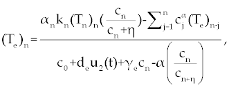
Now for solving optimization problem (20), we should first solve system (21-23) with some initial values of Tn, Te and C. Here, to be consistence with other results in (16,17), we start with Tn=1510, Te=10 and C=10000. Then, by finding the value  and plugging into the system (17-19), instead of u1(t) and u2(t), we are ready to solve 12 this system with the same starting point Tn, Te and C as above. Similar discretization method that we have done for FDE system (1-3) can be applied here for system (17-19) to get and plugging into the system (17-19), instead of u1(t) and u2(t), we are ready to solve 12 this system with the same starting point Tn, Te and C as above. Similar discretization method that we have done for FDE system (1-3) can be applied here for system (17-19) to get |
| |
 |
| |
 |
| |
 |
| |
| Now by simple calculation on (24-26), we get the following recursive formula. |
| |
 |
| |
 |
| |
 |
| |
By solving this system for some customary time, say t∈[0,1], we arrive at the new point Tn, Te and C. Then, this new set of values will serve as new starting point with initial values λ1(tf)=−B4, λ2(tf)=0 and λ 3(tf)=−B3 for solving system (21-23), in the next iteration, to find a new optimal value of . These iterations will continue up to the time t=250 (days). Indeed, using MATLAB™ to solve these two joint systems (27-29) and (21-23), as the solution of optimal problem (20), the results are illustrated in figures 2- 9 for different values of fractional derivative 0.90<α≤1. The results of patients A and B for α=1 (classical ODE) are shown in figures 2, 4, 6 and 8. These results are the same as in reference [2]. Figure 2 compares the behavior of CML cell population for one control (u1) as well as two controls (u1 and u2). For a more aggressive case of cancer (as for patient A) the CML cell count is significantly lower after treatment with combination therapy as compared to treatment by targeted therapy alone. For a less aggressive case (patient B) in figure 4, it may suffice to treat with one drug alone as the outcome is similar for single drug therapy and combination therapy. However, the CML plot of patient A is shown in figure 3 for α=0.95, which is different from figure 2. . These iterations will continue up to the time t=250 (days). Indeed, using MATLAB™ to solve these two joint systems (27-29) and (21-23), as the solution of optimal problem (20), the results are illustrated in figures 2- 9 for different values of fractional derivative 0.90<α≤1. The results of patients A and B for α=1 (classical ODE) are shown in figures 2, 4, 6 and 8. These results are the same as in reference [2]. Figure 2 compares the behavior of CML cell population for one control (u1) as well as two controls (u1 and u2). For a more aggressive case of cancer (as for patient A) the CML cell count is significantly lower after treatment with combination therapy as compared to treatment by targeted therapy alone. For a less aggressive case (patient B) in figure 4, it may suffice to treat with one drug alone as the outcome is similar for single drug therapy and combination therapy. However, the CML plot of patient A is shown in figure 3 for α=0.95, which is different from figure 2. |
| |
| As we can see in figure 2, with just one treatment u1, the CML cells increase to their lower bound 0.8 after 250 days. While in figure 3, which shows the results for our FDE model, these cells increase to the value 0.4. With the same comparisons in figure 2, when we have both treatments u1 and u2 the increasing slop of CML is lower than the slop for this cells in figure 3. We claim that the results found in our FDE model is closer to the nature of the drug treatment than the results found by ODE contra parts. However, this claim should be verified by the clinical treatment data. |
| |
| The CML plot of patient B is shown in figure 5 for α=0.95, which is again different from the plot in figure 4 for the same patient B using the classical ODE. In figure 6, there is not much difference in Tn evolution over time with or without drug therapy. Under targeted therapy, immune response is not compromised due to drug dosing. The Tn plot of patient B for fractional derivative α=0.95 is shown in figure 7, which is again different from the classical ODE plotted results in figure 6. These different are clear from the slops of the curves Tn in both figures. |
| |
| Finally, we see in figure 8 for patient B, whose cancer is of a less aggressive nature, that Te cell response is enhanced when treated only with u1. Using our FDE model, the similar results for patient B plotted in figure 9 with fractional derivative α=0.95. As we can see in figures 8 and 9, there is no significant different between the results whenever we have no treatments or both treatments u1 and u2 are on. However, for one drug treatment u1, in the case of classical ODE model the maximum of Te will be 24, while in FDE model this maximum will be 38. After these maximum, in both cases, Te will converge to zero. |
| |
| We claim that the results of figures 3, 5, 7 and 9 are more consistent with the nature of drug therapy. We emphasis, one reason for the accuracy of our FDE model is the non-local property of fractional derivative. This means that the next state of a system not only depends upon its current state but also upon its historical states starting from the initial time. To see this, pay attention to the summation terms in right hand side of system (27-29). However, as we have said above, this claim should be verified by more clinical treatment data. |
| |
| Conclusion |
| |
| In this article, we have studied a mathematical model with fractional order derivatives as a dynamic system for presenting the transaction between body immunology and drug variable. We have introduced a three cells population model describing the interaction between the CML and the naive T cells together with the effector T cell population, without any treatment, in the form of FDE. As we have seen, the local stability analyses of the fixed points for this FDE system were the same as its counterpart ODE system. These analyses were agreed with numerical results of discretized FDE system using Grunwald-Letnikov method. As we have expected the tumor cell population were increasing up to its maximum values by a positive initial value. Hence, a more reliable FDE system with chemotherapy treatment was considered. In order to find the best amount of medicine on which the tumor cell population, the naive T cells and the effector T cell population, decreasing we conducted a optimal control. The drug optimized dose is resulted from targeted therapy and broad cytotoxic therapy. We could adapt the same existence and characteristic optimal control theorems as in ODE systems for our FDE system. We claim, due to the non-local property of FDE, the results found by this system were more accurate as we compare to the results found by counterpart ODE models. Of course, this claim should be verified by more clinical treatment data. |
| |
| Here, we should emphasis that by choosing the small values of α∈[0,1] , we will encounter to the larger amount of error in calculations. In FDE models that we have introduced here, experimentally, we have found that the best value of α for the best results is 0.95. |
| |
| Acknowledgement |
| |
| This work was supported by Health Policy Research Center, Shiraz University of Medical Sciences |
| |
| |
| References |
| |
- Faderl S, Talpaz M, Estrov Z, O’Brien S, Kurzrock R, et al. (1999) The biology of chronic myeloid leukemia. N Engl J Med 341: 164-172.
- Nanda S, Moore H, Lenhart S (2007) Optimal control of treatment in a mathematical model of chronic myelogenous leukemia. Math Biosci 210: 143-156.
- Deininger MW, Goldman JM, Melo JV (2000) The molecular biology of chronic myeloid leukemia. Blood 96: 3343-3356.
- Deininger MW, O’Brien SG, Ford JM, Druker BJ (2003) Practical management of patients with chronic myeloid leukemia receiving imatinib. J Clin Oncol 21: 1637-1647.
- Deininger MW, Druker BJ (2003) Specific targeted therapy of chronic myelogenous leukemia with imatinib. Pharmacol Rev 55: 401-423.
- Van Rhee F, Szydlo RM, Hermans J, Devergie A, Frassoni F, et al. (1997) Long-term results after allogeneic bone marrow transplantation for chronic myelogenous leukemia in chronic phase: a report from the Chronic Leukemia Working Party of the European Group for Blood and Marrow Transplantation. Bone Marrow Transplant 20: 553-560.
- Baccarani M, Martinelli G, Rosti G, Trabacchi E, Testoni N, et al. (2004) Imatinib and pegylated human recombinant interferon-alpha2b in early chronic-phase chronic myeloid leukemia. Blood 104: 4245-4251.
- Kano Y, Akutsu M, Tsunoda S, Mano H, Sato Y, et al. (2001) In vitro cytotoxic effects of a tyrosine kinase inhibitor STI571 in combination with commonly used antileukemic agents. Blood 97: 1999-2007.
- Topaly JW, Zeller J, Fruehauf S (2001) Synergistic activity of the new ANL-specific tyrosine kinase inhibitor STI571 and chemotherapeutic drugs on BCR-ABL-positive chronic myelogenous leukemia cells. Leukemia 15: 342.
- Thiesing JT, Ohno-Jones S, Kolibaba KS, Druker BJ (2000) Efficacy of STI571, an abl tyrosine kinase inhibitor, in conjunction with other antileukemic agents against bcr-abl-positive cells. Blood 96: 3195-3199.
- Fokas AS, Keller JB, Clarkson BD (1991) Mathematical model of granulocytopoesis and chronic myelogenous leukemia. Cancer Res 51: 2084-2091.
- Adimy M, Crauste F, Ruan S (2005) A mathematical study of the hematopoiesis process with applications to chronic myelogenous leukemia. SIAM J Appl Math 65: 1328-1352.
- Afenya EK, Bentil DE (1998) Some perspectives on modeling leukemia. Math Biosci 150: 113-130.
- Moore H, Li NK (2004) A mathematical model of chronic myelogenous leukemia (CML) and T cell interaction. J Theor Biol 227: 513-523.
- Einstein A (1998) Mount Sinai School of Medicine. Annual Publication of the American Institute of Physics.
- Podlubny I (1999) Fractional differential equations, New York: Academic Press Inc, 368.
- Oldham KB, Spanier J (1974) The fractional calculus, New York: Academic Press Inc, 234.
- Matignon D (1996) Stability results of fractional differential equations with applications to control processing, in: IMACS, IEEE-SMC, Lille, France, 963.
- Borrelli R, Coleman C (1998) Differential Equations: A Modeling Perspective. Wiley, New York.
- Fister KR, Lenhart S, McNally JS (1998) Optimizing chemotherapy in an HIV model. Electron J Differential Equations 32: 1-12.
|
| |
| |
 ,
, ,
,
 ,
, ,
, .
. ,
, ,
, ,
, ,
, ,
, .
.


 ,
,


 ,
, ,
, .
. ,
, ,
, .
. ,
, ,
, .
. ,
,
 are given. Then there exist adjoint variables λi for i=1,2,3 and 4 that satisfy to the following system


