Dynamic Generation Expansion Planning of Reliability Constraints Effects
Received: 30-Sep-2015 / Accepted Date: 13-Oct-2015 / Published Date: 15-Oct-2015
Abstract
In this paper, a new method to solve Dynamic Generation Expansion Planning (DGEP) problem and transfer lines is presented. A new model for DGEP with several targets and many constraints is provided. In this method, genetic algorithm with decimal coding to solve development-programming problem is presented. In addition, the influence of reliability constraints on programming results is studied. The performance of the suggested method of power system typical is considered, too. Some of the main features of this work it is distinguished from previous works considering the cost of important fuel importance of distributed generation sources with the construction and study of the effect of reliability constraints.
Keywords: Dynamic generation expansion planning (DGEP); Genetic algorithm; Distribution generation (DG); Reliability; Wind farms
Introduction
The objectives of programming for the production development consist of determination of necessary units for construction, their construction timing, amount of productivity for purpose of minimizing total cost company (including fix cost and production).
Therefore, key to solution of GEP optimum problem was equivalent to the obtaining of optimum decision-making vector, such that object function has been reached a minimum under several limitations. The main reasons for consideration of renewable energies were the environmental problems and fuel crisis in the world including diffusion limitation of greenhouse gases especially CO2 gas. Generally, although renewable energies such as wind, water, sun and geothermic were rather expensive, and they have restricted due to their availability, but there have been increasingly interested in development of this resource kind to minimize environmental effects and the risk of absolute dependency on finite energy resource. In dynamic programming for the development of product, load changes determined within the limits of specific timing, for example perennial, and other constraints during this period such as fuel states, etc., the optimization problems must be solved somehow in any instant of time these limitations be considered according to limitations and constraints set. And during this time interval, the total spending cost has been reduced to a minimum. He YQ [1] suggested a smart system in dynamic programming algorithm so that combine many of meaningful processes in decision-making algorithm section. David AK [2] combined smart system with dynamic programming in order to decrease the dimensions of states space. It is possible to model the large dimension problems. David AK [3] presented a smart system with phase sets for optimum development programming that is extended mode of introduced method in reference [2].
In this article, how to plan the development of production with the provisions GEP reliability and with regard to the limitation of carbon dioxide emission is presented. Given that dynamic planning period is divided into several planning horizon.
Dynamic Generation Expansion Planning Model
Objective function
The generation-transmission equip sequence is described as a network G= (N, A), where N is the set of the nodes and A is the set of transmission lines. The ΔXlijt is a node (a point of demand and/or supply of energy), and the arc (i, j)∈ A is a transmission line, q∈Θ is a generation unit and t ∈T is a fossil fuel. T is the set of periods in the planning horizon where t ∈T is a time period.
Some decision variable are present in the DGEP model: ukt is the voltage phase angle at node i, Giqt is the generation amount (MW) of unit type q at node i in period t, niqt is the number of new units of type q at node i in period t, xiqt is the additional capacity (MW) of unit type q at node i in period t‚ ΔXlijt is the additional transmission capacity (MW) in arc (i,j) in period t‚lijt is the number of new circuits on arc (i,j) in period t‚ukt is the imported fuel (units) of type k in period.
In this problem, we considered minimization of total cost as object function. Total cost included development and exploitation cost of new units, establishment cost of new transfer lines, import fuel cost and disadvantage arise from fuel price changes. This amount defined as follow:
1) Development and exploitation cost of generation units in governmental network and cost pertain to transfer lines:
 (1)
(1)
Where d is the discount rate, ICiqt is the investment cost ($/MW) of a unit of type q at node i in period t, GCiqt is the generation (operation and maintenance) cost ($/MW) of a unit of type q at node i in period t and Cijt is the cost ($/MW) for new transmission capacity in arc (i,j) in period t.
2) Imported fuel cost:
 (2)
(2)
Where Vkt is the cost ($/unit) of imported fuel of type k in period t.
3) Energy price risk: This component showed the damage caused by fuel price changes during the development process.
 (3)
(3)
Where giqt is the total generation amount (MW) in unit of q kind in node i and period t and Skit is an expected coefficient of variation in prices of fuel type k in period t. According to defined components, fitness function determined as follow.
 (4)
(4)
Penalty was factor, if necessary, a number of existing limitation added to dominator of object function and dependent to violation of the limitation encompassed magnitude. The K coefficient was fixed value that can be used to prevent from small value of fitness function. Therefore, the aim of problem was maximization of fitness function.
Limitations
In DGEP, there are some limitation represented as follows:
1) Limitations of power balance in the network, transmission powers of lines and generation capacity of units: Finding generation power of units and transitory power of lines, the optimum dispersed load DC has been done via linear programming method. Therefore, we can write following relations based on DC load dispersion:
2) The amount of fuel in place
3) The development capacity of production and lines
4) Minimum and maximum reserve for generation
5) The limitation of emission rate of CO2 gas
6) Reliability constraints LOLP and LOEE have been considered as reliability indexes and should be met following conditions LOEE index defined as EENS-total energy on demand ratio.
Continuity Equivalent Load Curve and Equivalent Energy Function
Ai load curve for index calculation method of reliability a lot of time there. Convolution ELDC concepts and principles. Expressed by this method is equivalent to the energy function. EEF method has high computational accuracy and speeds are usually used for large systems in products description. The method for calculation of the reference index LOLP and EENS (1) is described.
 (5)
(5)
 (6)
(6)
Application Of GA For Solving Proposal Model
Although binary codification is conventional in genetic algorithm, but real and decimal coded genetic algorithms have been also used to solve some problems in [4-7] respectively. The new method regarding to solving of development programming problem was based on genetic algorithm with real coding. In this algorithm, each of people for any timing period was a vector that defined in the form of Figure 1. In this field, we have 4 distich, coincidental and variable groups. N indicates the number of new generation unit. I indicate the number of new circuit. Therefore, we divide variables into 2 groups and use the classified mutation operator to apply the accidental variations. In the aforementioned field, n and I are integer values. Thus, the intended chromosome length for any of people determine by following relation [8-10]:
 (7)
(7)
The Implementation Of Suggestive Method And Their Application On Specimen System
If we want to show the capabilities of the method, we should investigate the result of implemented method on the specimen power system. We select the Mexican inter connected power system in the level of region to carry out the suggestive method. The network information is based on available information in [4]. In 2005-2014 years scheduled the scheme that divided to two years periods. The base year was 2004 and the existing capacity, load peak and installed reservation in the system were 41443 MW, 36037/39 MW and 15% respectively. This system consisted of 7 nodes, 7 branches and 8 generation unit kinds with 4 fuel types. Generational technologies in system toward increasing capacity include: combined cycle modules (CC), coal units, nuclear, gas turbines (TG), wind farms, geothermal and hydro units. The non-renewable fuel types include: coal, gas, oil, and uranium. The respective information concerning power system has presented in Tables 1-6.
| Node | Steam | CC | TG | Coal | Nuclear | GEO | Wind | Hydro |
|---|---|---|---|---|---|---|---|---|
| 1 | 2092 | 496 | 898 | |||||
| 2 | 1035 | 1535 | ||||||
| 3 | 1265 | 3218 | 1488 | 2600 | 66 | |||
| 4 | 3466 | 577 | 597 | 2100 | 190 | 2783 | ||
| 5 | 1989 | 1449 | 292 | |||||
| 6 | 2380 | 1930 | 1365 | 40 | 6120 | |||
| 7 | 150 | 1045 | 277 |
Table 1: Existing capacity (MW) by technology in the base year.
| TYPE | Capacity (MW) | F.O.R | Fuel |  consume |
Units |  CO2 E |
 Invest |
O&M |
Cng | |
|---|---|---|---|---|---|---|---|---|---|---|
| 1 | STEAM | 350 | 0.1 | Oil | 1.54 | Barrel | 0.795 | 166 | 494064 | 35 |
| 2 | CC | 560 | 0.07 | Gas | 7.00893 | Mbtu | 0.359 | 80 | 525600 | 60 |
| 3 | TG | 184 | 0.1 | Gas | 10.43537 | Mbtu | 0.508 | 60 | 630720 | 48 |
| 4 | COAL | 350 | 0.08 | Coal | 0.46587 | TON | 0.957 | 260 | 252288 | 35 |
| 5 | NUCLEAR | 1506 | 0.05 | Nuclear | 2.68000 | GR | 0 | 386 | 105120 | 5 |
| 6 | GEO | 230 | 0.09 | Steam | 0 | TON | 0 | 212 | 191318.4 | 10 |
| 7 | WIND | 100 | 0.6 | Wind | 0 | NO | 0 | 200 | 52560 | 30 |
| 8 | HYDRO | 200 | 0.01 | Water | 0 | NO | 0 | 180 | 252288 | 50 |
Table 2: Type of units.
| Fuel | Units | Capacity |
Import Cost |
Prices CF |
|---|---|---|---|---|
| Oil | Barrel/day | 1742.27460 | 26.75 | 0.29 |
| Gas | Mbtu/day | 42630.45704 | 4.70 | 0.40 |
| Coal | Ton/year | 16800 | 33 | 0.05 |
| Nuclear | GR | 1000 | 2.1 | 0.025 |
Table 3: Fule type.
| Node | 2006 | 2008 | 2010 | 2012 | 2014 |
|---|---|---|---|---|---|
| 1 | 2873 | 3140 | 3473 | 3821 | 4135 |
| 2 | 3216 | 3542 | 3941 | 4382 | 4832 |
| 3 | 6673 | 7363 | 8293 | 9352 | 10511 |
| 4 | 7412 | 8302 | 9344 | 10423 | 11493 |
| 5 | 8762 | 9453 | 10298 | 11196 | 12069 |
| 6 | 6187 | 6890 | 7743 | 8617 | 9558 |
| 7 | 1229 | 1391 | 1604 | 1816 | 2072 |
Table 4: Peak load (MW) in each period.
| Origin | Destine | Capacity |
Fixed C |
Length (Miles) |
Cnl | |
|---|---|---|---|---|---|---|
| 1 | 2 | 300 | 3.903 | 176 | 0.1490 | 1 |
| 1 | 4 | 320 | 3.903 | 252 | 0.2 | 1 |
| 2 | 3 | 260 | 3.903 | 215 | 0.21 | 1 |
| 3 | 6 | 1000 | 3.903 | 231 | 0.0587 | 1 |
| 4 | 5 | 2900 | 3.903 | 232 | 0.0203 | 1 |
| 6 | 5 | 3800 | 3.903 | 280 | 0.0187 | 1 |
| 6 | 7 | 435 | 3.903 | 296 | 0.1728 | 1 |
Table 5: Inter-area links in the base year.
| Parameter | Rate (%) |
|---|---|
| Investment inflation | 3 |
| Operation inflation | 5 |
| Fuel inflation | 4 |
| Transmission inflation | 3 |
Table 6: Economical component.
| period | Units | Lines | ||||||||||
|---|---|---|---|---|---|---|---|---|---|---|---|---|
| node | Steam | CC | TG | Coal | Nuclear | GEO | Wind | Hydro | Origin | Destine | Number | |
| 1 | 1 | 1 | 2 | 1 | ||||||||
| 2 | 1 | 4 | ||||||||||
| 3 | 2 | 3 | 1 | |||||||||
| 4 | 3 | 6 | 1 | |||||||||
| 5 | 1 | 4 | 5 | |||||||||
| 6 | 6 | 5 | ||||||||||
| 7 | 6 | 7 | ||||||||||
| 2 | 1 | 2 | 1 | 2 | ||||||||
| 2 | 1 | 1 | 4 | |||||||||
| 3 | 2 | 2 | 3 | |||||||||
| 4 | 1 | 2 | 3 | 6 | ||||||||
| 5 | 2 | 4 | 5 | 1 | ||||||||
| 6 | 1 | 1 | 2 | 6 | 5 | |||||||
| 7 | 6 | 7 | ||||||||||
| 3 | 1 | 1 | 2 | 1 | 2 | |||||||
| 2 | 1 | 4 | ||||||||||
| 3 | 2 | 2 | 3 | |||||||||
| 4 | 1 | 2 | 3 | 6 | ||||||||
| 5 | 2 | 4 | 5 | |||||||||
| 6 | 1 | 2 | 6 | 5 | 1 | |||||||
| 7 | 1 | 6 | 7 | |||||||||
| 4 | 1 | 1 | 2 | 1 | 2 | |||||||
| 2 | 1 | 1 | 4 | |||||||||
| 3 | 1 | 2 | 2 | 3 | ||||||||
| 4 | 1 | 2 | 3 | 6 | ||||||||
| 5 | 1 | 1 | 4 | 5 | ||||||||
| 6 | 1 | 2 | 6 | 5 | ||||||||
| 7 | 6 | 7 | ||||||||||
| 5 | 1 | 1 | 1 | 1 | 2 | |||||||
| 2 | 1 | 1 | 4 | 1 | ||||||||
| 3 | 1 | 1 | 2 | 2 | 3 | |||||||
| 4 | 1 | 2 | 3 | 6 | ||||||||
| 5 | 1 | 1 | 2 | 4 | 5 | |||||||
| 6 | 1 | 1 | 2 | 6 | 5 | |||||||
| 7 | 1 | 6 | 7 | 1 | ||||||||
Table 7: A new generation units and transmission line addition case 1.
| Period | 1 | 2 | 3 | 4 | 5 |
|---|---|---|---|---|---|
| Reliability Index | |||||
| LOLP | 0.0194 | 0.0319 | 0.0257 | 0.0189 | 0.0706 |
| LOEE | 0.0011 | 0.0017 | 0.0012 | 0.0008 | 0.0035 |
Table 8: Reliability indexes for case 1.
| period | Units | Lines | ||||||||||
|---|---|---|---|---|---|---|---|---|---|---|---|---|
| node | Steam | CC | CC | Coal | Nuclear | GEO | Wind | Hydro | Origin | Destine | Number | |
| 1 | 1 | 1 | 2 | 1 | ||||||||
| 2 | 1 | 4 | ||||||||||
| 3 | 2 | 3 | 1 | |||||||||
| 4 | 3 | 6 | 1 | |||||||||
| 5 | 1 | 4 | 5 | |||||||||
| 6 | 6 | 5 | ||||||||||
| 7 | 6 | 7 | ||||||||||
| 2 | 1 | 2 | 1 | 2 | ||||||||
| 2 | 1 | 1 | 1 | 4 | ||||||||
| 3 | 2 | 2 | 3 | |||||||||
| 4 | 1 | 1 | 2 | 3 | 6 | |||||||
| 5 | 2 | 4 | 5 | 1 | ||||||||
| 6 | 1 | 1 | 1 | 2 | 6 | 5 | ||||||
| 7 | 6 | 7 | ||||||||||
| 3 | 1 | 1 | 1 | 2 | 1 | 2 | ||||||
| 2 | 1 | 4 | ||||||||||
| 3 | 2 | 2 | 3 | |||||||||
| 4 | 2 | 3 | 6 | |||||||||
| 5 | 2 | 4 | 5 | |||||||||
| 6 | 1 | 2 | 6 | 5 | 1 | |||||||
| 7 | 1 | 1 | 6 | 7 | ||||||||
| 4 | 1 | 1 | 2 | 1 | 2 | |||||||
| 2 | 1 | 1 | 1 | 4 | ||||||||
| 3 | 1 | 1 | 2 | 2 | 3 | |||||||
| 4 | 1 | 1 | 2 | 3 | 6 | |||||||
| 5 | 1 | 1 | 1 | 4 | 5 | |||||||
| 6 | 1 | 2 | 6 | 5 | ||||||||
| 7 | 6 | 7 | ||||||||||
| 5 | 1 | 1 | 1 | 1 | 1 | 2 | ||||||
| 2 | 1 | 1 | 1 | 4 | 1 | |||||||
| 3 | 1 | 1 | 1 | 2 | 2 | 3 | ||||||
| 4 | 1 | 1 | 2 | 3 | 6 | |||||||
| 5 | 1 | 1 | 1 | 2 | 4 | 5 | ||||||
| 6 | 1 | 1 | 1 | 2 | 6 | 5 | ||||||
| 7 | 1 | 1 | 6 | 7 | 1 | |||||||
Table 9: A new generation units and transmission line addition case 2.
| Period | 1 | 2 | 3 | 4 | 5 |
|---|---|---|---|---|---|
| Reliability Index | |||||
| LOLP | 0.0181 | 0.02 | 0.02 | 0.0091 | 0.0048 |
| LOEE | 0.001 | 0.001 | 0.001 | 0.0006 | 0.0002 |
Table 10: Reliability indexes for case 2.
| Unit | Steam | CC | TG | Coal | Nuclear | GEO | Wind | Hydro |
|---|---|---|---|---|---|---|---|---|
| Case | ||||||||
| 1 | 1 | 6 | 8 | 4 | 1 | 8 | 26 | 33 |
| 2 | 0 | 16 | 1 | 4 | 2 | 0 | 2 | 38 |
Table 11: Number of new units that must be added to network in whole programming duration.
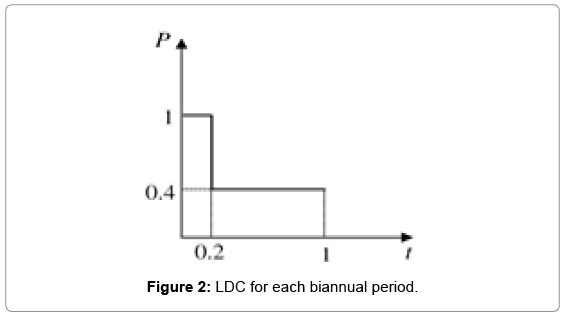
The limitation of emission CO2 gas in scheduled year has selected in 46000 TON. The minimum and maximum of reservation value in any period equated to 5% and 15% load peak respectively. The minimum and maximum of exploitation capacity in any unit kind estimated in 20%and 98% of total capacity and interest rate evaluated in 5%. LCD curve for each area as shown in step 3 is considered. In this curve, the horizontal axis per united on the basis of 2 years times limit and the vertical axis per united in second year of 2 years times limit with maximal load. This problem has a grant complication and broadness and therefore it can be solved by many of reliable functional and engineering hypothesizes. These suppositions have not caused any damage to generalization problem and is possible to solve it. They presented the main features of the model. The intended supposition for solving problem is as follow:
-The number of the available branches are equal to 7. That the development of transfer lines accomplish a long side of these branches routes. There aren’t a new route for the establishment of new lines. The capacity of additive line to any route is equal to available branch capacity in that route at primary conditions of system and prior to start of programming process.
-In regard to the limitation of generation units with renewable energies, it developed in many of certain areas. In order that it may be easier to study the effect of reliability constraint, we considered two type of indexes. Therefore we can carry out the suggestive method with each of under cases upon the sample system.
Case 1: without limitation of reliability and with limitation of CO2 emission.
Case 2: with limitation of reliability and with limitation of CO2 emission.
Before, we studied the results from suggestive method implementation for any of cases, we define following parameters for total duration of programming:
U cost: The sum of development and exploitation costs of generation unit, costs pertain to establishment of transfer lines, costs of imported fuel and loss caused by fuel price changes (total cost).
fixcu: The cost of creating the new units.
ECO2: The amount of imported CO2.
Fuel cost: The cost of imported fuel.
LOLP and LOEE indexes have considered as reliability indexes in the generational section. The EEF method used to calculate it. To obtaining of maximum values in each of these indexes. Their values calculated in base year by means of energy function method:
 We can use the obtained values in the year and select the maximum value for each of reliability indexes as follow:

The features of GA method for solving problem in any of two cases presented below:
The number of population: 50 people
The mutation rate (Pm): 0/01
The substitution rate (Pc): 0/9
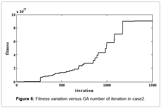
The criterions for completion of program execution are the convergence of fitness function and it’s unchangeable with increasing iteration number. In the cases, algorithm converged in 1500 iteration. The computer specifications and the time of program execution presented below.
Computer specification: RAM 4 GB, CPU 2.8 GHZ, PC, Pentium 4.
The average of execution time per cycle in genetic algorithm in any of two cases: 7.2 seconds
The average of EEF execution time for calculating reliability: 5 seconds
Although, EEF method calculated reliability indexes of the generation, especially large networks, quickly, but, it’s performance in any field in population and the number of iteration above genetic algorithm increased the dimensions of calculation and the time of program execution largely. Therefore, reliability constraints included in program and EEF performed for whole fields of population per 100 iteration at genetic algorithm in case 2. This value obtained from multiple genetic algorithm implementation and comparison with the results.
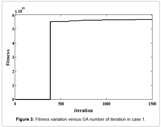
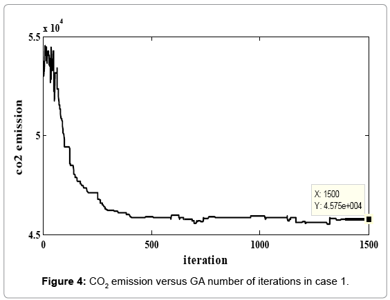
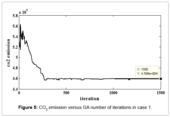
In Figures 2-6 we exhibit the way of fitness function variations for each of two cases. As you observed, genetic algorithm converge in 1500 iteration. In Tables 7-9, the number of added units to any node and the number of added branches to conduction system at different time of intervals have presented. The number of increasing branches in power system obtained for communication of load distribution and rising production and consumption and the limitation number of increased branches had been investigated. Reliability indexes for each case presented in Tables 8 and 10. In any case, the cost of new establishing units, emission rate of CO2 gas and cost of imported fuel have obtained. The development constraints (CO2 emission, the number of different unit, reservation…) in any two cases have been evaluated. We investigate the obtained value of reliability indexes in any case and observe that in some of periods doesn’t fulfill reliability constraints in case 1. (This values specified in respective tables). But we apply the offered method and include reliability constraints as error function in the problem of objective function in case 2 and fulfill this constraint. Figures 5 and 6 showed that emission rate of CO2 gas have decreasing order to meet fuel constraints. The limitation of dioxide carbon emission in cases 1 and 2 considered and declined its extent so that it fulfilled the anticipated extent (46000 Ton).


Tables 10 and 11 show the number of new units that must be added to network in whole programming duration (10 years) according to unit type in any of two planning cases. The condition of fuel limitation and cost of consumed fuel caused tendency toward renewable energies.
Considering the constraint of CO2 emission increased the number of unit with renewable energies and combinational cycle units and decreased coal units. Thus, this program fulfills the limitation of CO2 emission by means of units having less pollution percentage. In comparison case 1 with case 2, we observe that regarding reliability constraints in case 2 increase the number of new power plant in combinational cycle units while decrease winds power stations. The wind power station has most probability of forcible exit (FOR). Also, combinational cycle power plant has less FOR than other fossil power plant. Therefore it can be deduced that with consideration of reliability constraints in the problem, the program pressed towards the reduction capacity of power plants and the probability of forceful exit was high, in so far as reliability constraints estimated with least possible cost.
In case 2, the total cost will be increased accordingly. Indeed, it can be said that this different cost was due to making use of units with high reliability (small FOR) so that supply the reliability constraints. This constraints imposed great cost.
Conclusions
In this paper, we considered the performance of suggestive method in two different cases for development programming that allowed investigation the effect of reliability constraints and CO2 gas emission for manufacturing and exploitating of generational unit. We considered the results of implemental suggestive method and noticed that this method had a desirable performance in offering obvious pattern to the government towards oncoming development and it can be solved uncertainty greatly.
References
- He YQ, David AK (1995) “Advances in global optimization for generation expansion planning”, IEEE Proceeding-Generation, Transmission and Distribution, 142: 423-430
- David AK, Zhao R (1989) “Integrating expert systems with dynamic programming in generation expansion planning”, IEEE Transaction on Power Systems, 4: 1095-1100.
- David AK, Zhao R (1991) “An expert system with fuzzy sets for optimal planning”, IEEE Transactions on Power Systems, 6: 59-65.
- Meza JL (2006) “Multicriteria Analysis of Power Generation Expansion Planning”, Ph.D. Dissertation, Wichita State University.
- Jia NX, Yokoyama R, Zhou YC Kozu A (2000) “An Effective DP Solution for Optimal Generation Expansion Planning under New Environment”, IEEE Inter. Conf. on Power System Tech. 1: 37-42.
- Jia NX, Yokoyama R, Zhou YC, Kozu A (2000) “An Effective DP Solution for Optimal Generation Expansion Planning under New Environment”, IEEE Inter. Conf. on Power System Tech,1: 37-42.
- Raie A, Rashtchi V (2002) “using a genetic algorithm for detection and magnitude determination of turn faults in an induction motor, ” electrical engineering,84: 5.
- Jalilzadeh S, Kazemi A, MahdaviM, shayeghi H (2008) “Technical and economic evaluation of voltage level effect in transmission network expansion planning using GA”, Elsevier-Energy Conversion and Management 49: 1119-1125.
- Wang X, McDonald JR (1994) "Modern power system Planning", MCGRAW-HILL Publication.
- Shirley R, Kammen D (2015) “Energy planning and development in Malaysian Borneo: Assessing the benefits of distributed technologies versus large scale energy mega-projects”, Energy Strategy Reviews 8: 15-29.
Citation: Ghorbani A (2015) Dynamic Generation Expansion Planning of Reliability Constraints Effects. Innov Ener Res 4: 126.
Copyright: ©2015 Ghorbani A. This is an open-access article distributed under the terms of the Creative Commons Attribution License, which permits unrestricted use, distribution, and reproduction in any medium, provided the original author and source are credited.
Share This Article
Open Access Journals
Article Usage
- Total views: 10138
- [From(publication date): 12-2015 - Apr 27, 2024]
- Breakdown by view type
- HTML page views: 9411
- PDF downloads: 727


