A Holistic View of Finite Populations for Determining an Appropriate Sample Size
Received: 30-May-2019 / Accepted Date: 19-Jul-2019 / Published Date: 26-Jul-2019 DOI: 10.4172/2155-9910.1000272
Abstract
This study presents practical and easy-to-implement approaches for determining appropriate, or “safe” sample sizes for routinely conducted statistical surveys. Finite populations are considered holistically and independently of whether they are continuous, categorical or dichotomous. It is proposed that in routinely conducted sampling surveys variance-ordered categories of populations should be the basis for calculating the safe sample size given that the variance within a target population is a primary factor in determining sample size a priori. Several theoretical and operational justifications are presented for this thesis. Dichotomous populations are often assumed to have higher variances than continuous populations when the latter have been standardized and have all values in the interval (0 1). Herein, it is shown that this is not a valid assumption; a significant proportion of dichotomous populations have lower variances than continuous populations. Conversely, many continuous populations have variances that exceed the limits that are broadly assumed in literature for determining a safe sample size. Finite populations should thus be viewed holistically. A simple first step is to partition finite populations into just two categories: convex and concave. These two categories are relative to a flat population with a known variance as the threshold between them. This variance is used to determine a safe sample size for any continuous population with a flat or positive curvature, including approximately 20% of dichotomous populations. For all other populations the value of 0.25 is recommended for approximating the actual population variance as the primary parameter for sample size determination. The suggested approaches have been successfully implemented in fisheries statistical monitoring programs, but it is believed that they are equally applicable to other applications sectors.
Keywords: Statistical surveys; Sampling techniques; Finite populations; Sample size determination
Introduction
This study stems from the author’s experience in implementing sample-based data collection programs in the fisheries sector. In such situations the surveys are implemented on a routine basis with the purpose of systematically monitoring the exploitation of marine and inland fishery resources. A typical fishery statistical monitoring program consists of two sampling surveys that are conducted in parallel and are independent of each other.
In the first survey the target populations are fish landings made by different fleet segments, such as trawlers, purse seiners, small artisanal boats, etc. The reason for segmenting the boats by vessel type and fishing method is to form statistical strata in each of which fish production is more homogeneous with respect to species composition, quantities caught, fishing grounds exploited, etc. The objective is to estimate on a monthly basis the average daily harvest of a boat from each fleet segment separately. Landings populations are continuous with frequency distributions that are specific to the boat type and fishing method employed. For instance, the distribution of landings by trawlers or boats using traps is usually skewed and at times approximately normal. Landings by purse seiners targeting small pelagic fish are at times U-shaped since in this type of fishery there are days of large catches and others of little or no catch at all. Consequently, these data tend to be thin around the mean and denser near the lower and upper boundaries of their range. Small-scale fisheries that are practiced by small craft have distributions of varying positive curvature; at times the distribution can be flat (or orthogonal) without noticeable peaks within the data range.
The second survey concerns the level of activity of boats. This is expressed by the probability that a boat of a fleet segment is active (i.e. fishing) on any given day. This probability is subsequently used to estimate the monthly fishing effort of a fleet segment (i.e. total days at sea during a month). There exist several sampling scenarios for estimating the level of activity and the respective target populations are specific to the sampling scheme in use. For instance, one scenario is to sample at random the activity state of boats; this state is conventionally expressed by 1 if the boat is found fishing and by zero if it is not. In this case the target population is dichotomous and its proportion p is equivalent to the probability of a boat being active. Another approach is to sample boats at random on a weekly basis and record the number of days fishing over the past week. In this case the population is categorical and consists of eight values (0 to 7) that appear with varying frequencies.
The introductory information given above indicates that in routinely conducted fisheries surveys the target populations are of varying types: continuous for landings (comprising skewed, approximately normal, flat and U-shaped data) and dichotomous or categorical for boat activity. These populations are stratified by boat type and fishing method and by coastal zone, since the latter can also affect the species composition and the quantities caught. Thus, in a typical fisheries statistical monitoring program sampling operation apply to many statistical strata whose number can be as big as 200. It should be added here that in all cases the populations are finite and their respective size is known with good accuracy.
During the planning phase of a fisheries sample-based program it is essential to set-up data collection norms and standards for each stratum in the statistical area. The most important task is to determine the appropriate sample size for each stratum, separately for landings and for boat activities, bearing in mind that such settings may vary from month to month due to the dynamics of the fisheries populations under study.
The determination of an appropriate sample size is known to be a key factor in all types of sample-based surveys. Data collection schemes in large-scale statistical program demand that the safe sample size is determined on an a priori basis at the beginning of each reference period (e.g., each month) and for each target population of the survey. Various approaches for this a priori determination is extensively discussed in the literature; a plethora of studies have been conducted to examine the use of Cochran’s formula [1], either in its original form or with modifications based on specific methodological and/or operational requirements. Although this introductory section is not intended for methodological presentations, Cochran’s formula for safe sample size merits some brief discussion since its parametrization is the focus of the present study. As shown in Section 2 this formula derives directly from the Central Limit Theorem and has the following form:

where n is the resulting sample size, t is the abscissa of the normal curve that cuts off a total area of α at the tails, σ2 is the population variance and ε is the maximum error that the survey planner is willing to tolerate.
A typical value for t is 1.96 which corresponds to an alpha level of 0.05. In practical terms this means that when the sample size is calculated from the above formula 95% of the sampling operations are expected to yield a sampling error that is lower than ε .
An immediate observation on the above formula is that the population variance is unknown. Approximating the population variance with the sample variance requires some extent of preliminary sampling which defeats the idea of a priori determination of sampling requirements. In dichotomous populations this difficulty can be overcome by replacing the population variance with the “pessimistic” constant 0.25 which is the maximum variance in dichotomous populations and occurs for population proportions that are equal to 0.5. When the population proportion is not 0.5 the approach leads to oversampling, but most users are quite willing to accept this fact since it provides an even safer sample size and at the same time it mitigates the impact of the alpha level described earlier.
When analyzing continuous data, the recommended actions for parametrizing the sample size formula are less straightforward. One would expect that using again a pessimistic maximum for the variance, a good and practical approach that works well with dichotomous data, could also apply to continuous data. Instead, most case studies in literature focus on the target population in hand and attempt to closely approximate the population variance using hypotheses and educated guesses.
For instance, it has been suggested that the population variance can be estimated with a reasonable degree of accuracy [2,3]; it has also been hypothesized that the population is approximately normal and that its variance can be approximated using a seven-point scale that includes six standard deviations [4]. However, in surveys that are routinely conducted, such approaches are not always feasible. As described earlier there are several sub-populations resulting from stratification schemes that combine geographical and technical criteria and that their number could well be as big as 200. In such situations it is impractical to conduct a priori approximations of the variances for each of these 200 sub-populations on a monthly basis, even in the unlikely event that statisticians are present during the production phase of a routinely conducted statistical monitoring program. Furthermore, the assumption that a continuous population is normal or approximately normal is not always valid: it was seen earlier that continuous data (such as fish landings) come in various forms and shapes and apart from some knowledge about the general configuration of the elements, not much is known in advance about the variance in the data. It is the author’s view that in routinely conducted surveys the approximation of variances for each target population separately is not a feasible approach.
Here, it is advocated that in routinely conducted sampling surveys the parametrization of the sample size formula should always be based on the “pessimistic” approach, whereby a maximum variance replaces the population variance in the formula. To achieve this, we need to take a holistic view of the variance, irrespective of the population being continuous, dichotomous or categorical. We suggest that transforming finite populations into standardized ones (i.e., mapping the original elements onto the interval (0 1) allows all populations of a given size to be ordered on the basis of variance and partitioned into two major categories, each with known maximum variance. We can then use the “pessimistic” approach by means of which the variance in the sample size formula is replaced by the maximum variance of the respective population category.
An example of such a holistic approach is illustrated in Figure 1 with standardized populations having values within the interval (0 1) and ordered based on variance. The threshold line representing a flat population corresponds to a variance of and divides all finite populations of same size N into two major categories:

Figure 1: Standardized populations sorted in ascending order of variance and the two major categories of populations based on σ2 = 1/12 .
(i) Populations with variances ≤ 1/12.
(ii) Populations with variances >1/12 and ≤ 1/4.
The first (upper) category is conventionally referred to as “convex” and includes all continuous populations with flat or positive curvatures, including categorical populations whose peak frequencies are around the mean. Surprisingly enough, this category also includes dichotomous populations with proportions of p<0.09 or p>0.91 (this last property is proved in the annex).
The second category is referred to as “concave” and includes continuous populations with negative curvatures (i.e., U-shaped populations), categorical populations with peak frequencies near the boundaries and dichotomous populations with proportions 0.09 ≤ p ≤ 0.91.
This introductory section concludes with a brief description of the main body of the document.
Section 2 provides definitions and notations and describes the application of a population standardization process to map a finite population to values in the interval of (0 1). Next, all standardized populations of the same size are ordered by the variance and two major population categories are identified. The final step determines safe sample size for each category.
Four case studies are included that show the practical application of the proposed approach. All datasets contain actual data collected in the field and specifically from the fisheries statistical programs that operate in Qatar, the UAE, Lebanon and Algeria. All data have been standardized to take values within the interval (0 1) using the standardization method presented at the beginning of the section.
Section 3 opens a discussion regarding the proposed approaches. Several conclusions are drawn in Section 4.
The methodologies presented in Sections 2 and 3 are further analyzed in the annex in the form of mathematical proofs for most propositions. This was done with the purpose of providing the theoretical basis for the categorization of populations using as criterion the variance. Most of the mathematical proofs in the annex concern the very questions of: (i) how the variance increases or decreases when the population elements change positions and (ii) what the global minimum and maximum variances in standardized populations of a are given size. Admittedly the proofs of some known and/or self-evident facts might seem superfluous but the author has opted to include them nevertheless, more for his own reassurance than that of the reader.
Materials and Methods
The topics in this section are presented in the following order:
• Assumptions, definitions, and conventions concerning finite populations;
• Transformation method of a finite population into a standardized population;
• Description of variance-ordered standardized populations and the pessimistic approximation of variances;
• Examples of error-prediction functions;
• Examples of safe sample size determination.
Assumptions, definitions and conventions
All populations in this study are finite, have a known size (N), and contain at least two elements that are different from each other. The population elements are denoted by an indexed variable (i=1, …, N). The population mean is denoted by. Without any loss of generality, the population elements are assumed to be arranged in increasing order so that for all i=1, …, N-1. Hence, there is always a minimum element and a maximum element.
Herein, there is a distinction between the terms “curvature” (or “shape”) and “configuration”: the former refers to the form of the frequency distribution of the population while the latter refers to the positioning of the population elements within the interval defined by its boundaries. An example of this distinction is shown in Figure 1 that illustrates standardized populations (with elements between 0 and 1), which are ordered by the variance. Let us examine the U-shaped population shown near the bottom. The curvature of the population is described by its frequency distribution, whereas the configuration of population elements is described (just above it) by the positioning of its elements within the interval (0 1).
For a random sample of size n denoted as (k=1, …, n) with a sample mean of the relative error is computed as follows:
 (1)
(1)
It is recalled that are the minimum and maximum elements respectively.
Herein, all populations in the study are assumed to have been transformed into standardized populations as shown in the following section in order to simplify the discussion of the relationship between sample size and relative error.
Standardized populations
Using the minimum and maximum elements Y1, YN the finite population, Yi, described above can be transformed into a standardized population, Xi, according to the following formula:
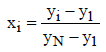 (2)
(2)
The resulting standardized population has the following basic properties (these are self-evident and do not require a formal proof):
(a) 1 x= 0 xN =1 0 ≤ Xi ≤ 1i=2, ….N-1.
(b) Mean of the standardized population is 
(c) Sample elements are mapped onto standardized sample elements which have a sample mean of

(d) From (a), (b) and (c), it follows that the relative error given in (1) is also equal to:  (3)
(3)
Property (d) indicates that the relative error can be measured directly from the unitless standardized population generated according to (2). An illustrative example of this property is provided in the annex.
(e) If σ2 is the variance of a standardized population then, according to the central limit theorem, for error in (3) we will have:
 (4)
(4)
where n is the sample size and t are the abscissa of the normal curve that cuts off a total area of α at the tails. To simplify the calculations, we assume that the populations are large enough, so that formula (4) need not contain the Finite Population Correction factor (FPC).
Assuming the equal sign in (4) and solving the equation for n, we obtain Cochran’s general formula for a safe sample size:
 (5)
(5)
Based on properties (d) and (e), it can be concluded that sampling aspects can be examined with respect to standardized populations only. The propositions following, (f)-(j), hold for all standardized populations of size N and are proved in the annex.
(f) When an element is moved away from the mean and toward either of the two boundaries, 0 and 1, the variance of the population increases.
(g) When an element is moved toward the mean, the variance of the population decreases.
(h) In standardized populations, the variance has a global maximum of  .This maximum occurs in dichotomous populations with a proportion of p=0.5 and when the population size, N, is an even number. When N is an odd number this maximum is slightly lower, as shown in Proposition 2 in the Annex, but the difference between the two maximum values is quite negligible so that the value of 1/4 is accepted in all cases.
(i) The variance has a global minimum of  which is practically zero for large values of N.
(j) There is a unique “flat” standardized population that does not contain regions of high or low element densities. The variance of this type of population is 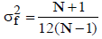 and has a limit of 1/12 for large values of N.
Convex and concave populations
Once all populations have been standardized and ordered by their variance, σ2 , they can be partitioned into two major categories based on the “flat” variance, σ2f , defined in property (j) above as follows:
Convex populations: 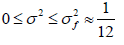 (6)
(6)
Concave populations: 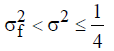 (7)
(7)
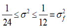
The classification for convex populations relies on the use of flat variance,σ2f , as a pessimistic substitute for the variances of all convex populations, including those with Gaussian and Laplacian distributions and those with slight positive curvatures, etc. Likewise, the global maximum,  , can be used as a pessimistic substitute for the variances of all concave populations including those that have U-shaped distributions and those that are dichotomous without high or low proportions. Cochran and Krejcie and Morgan [1,5] have used σ2max for dichotomous populations. However, as shown in Section 3, not all dichotomous populations have high variances and not all continuous populations have low variances. Therefore, in the case where the researcher considers only two population categories, it would be more accurate to use the term “convex” for populations with variances between 0 and 1/12 inclusive and “concave” for populations with variances that are higher than 1/12 and lower than or equal to 1/4.
The pessimistic variance approach using two major population categories (i.e., convex and concave) is efficient and easy to implement. The author has been involved in the design and implementation of routinely conducted fishery surveys in several countries, and in his experience, the use of these two major categories is robust and durable. It should be noted here that fishery surveys involve simultaneous dealing with various population types: normal (or about normal), convex with a slight curvature, flat, U-shaped, and dichotomous. The examples presented in this section are based on actual data compiled from the field.
Therefore, it is recommended that this approach is used as a first step when determining safe sample size, considering that it could later be replaced by a more refined categorization scheme if this new scheme is equally reliable, robust, and durable. One such case is illustrated in Figure 1: a thin line representing a variance of 1/24 (which is half of the flat variance 1/12) further divides the convex populations into those that have normal or relatively sharp curvatures and those with zero or slightly positive curvatures. This shows that more refined classifications of populations yield safe sample sizes that are more economical because the pessimistic variances were designed to be applicable to smaller population categories. As an example, if the population size, N, is large enough to permit the use of the limit-values for variances, the following refined categorization can be used:
Convex with a normal or relatively sharp curvature:
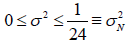
Convex with no curvature or a slight curvature:
Concave: 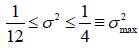
It should be noted that categories (i) and (ii) also contain dichotomous populations with proportions in the ranges of p<0.09 or p>0.91 while category (iii) contains U-shaped continuous populations and dichotomous populations with proportions in the range of 0.09 ≤ p ≤ 0.91.
As mentioned earlier, the use of two major categories, convex and concave, as described by (6) and (7), is recommended here. The subdivision of convex populations into two sub-categories, (i) and (ii), is done in order to show that the general approach presented here is flexible enough to accommodate the use of more refined categorizations if it can be justified by available information about the shape of the target populations.
Error fluctuation and sample size
In Section 2.2, it was shown that formula (5) for determining the safe sample size is a rearranged form of formula (4), in which the error, ε , is a function of the sample size, n. This error-prediction function envelops most of the error points resulting from the varying sample size with some exceptions depending on the selected alpha level, which is represented by t value in the formula. For instance, for an alpha level of 0.05 (or 5%), it is expected that if sampling is repeated 100 times, in 95 cases the relative error ε will be lower than the allowable error margin (such as 0.1 and 0.05). This expectation is based on the actual population variance that appears in formula (5). Evidently, when the population variance is substituted by a higher (e.g., pessimistic) value, the sample size will increase, with increasing proportion of “good” occurrences for the error ε .
As the sample size increases, the error decreases and its fluctuation are mitigated. In case of large samples and when the sample size continues to increase, the error curve begins to converge toward zero.
In the following examples, the sample size, n, ranges from 1 to 500. For each sample size, a random sample is taken and its mean is combined with the population mean to derive the relative error, given in formula (3). The series of plotted errors form an oscillating curve that becomes smoother as the sample size increases. In each example, the three error-prediction curves defined for categories (i)-(iii) (as defined in Section 2.3) are plotted together in order to illustrate how efficiently each one envelops the actual error fluctuation. As mentioned earlier, this efficiency (or lack thereof) depends on the pessimistic value that is chosen to represent the population standard deviation in (4).
In the error plots presented for the following examples, the horizontal axis represents the ratio, log(n)/log(N), where N is the population size, rather than the sample size, n. This is done simply for the sake of convenience because plotting the error as a function of sample size has a hyperbolic shape so much that the error function is very close to the axis and, thus, is blurred and difficult to visualize. Conversely, with a logarithmic scale, the plot is magnified horizontally and the curve takes on an exponential shape that is easier to analyze. This type of graphical representation is only for plotting purposes and it does not affect the methods, or the formulae used.
Illustrative examples of error prediction
Example 1: Figure 2 illustrates an application of the error-prediction formula (4) to a standardized population of fish landings by trawlers, which is known to be approximately normal. The function represented by the dotted line was parametrized for populations that are normal or sharper than normal (i.e., those in category (i) as defined in Section 2.3). The pessimistic variance was set to 1/24 and the acceptable margin of error was chosen to be 0.05.

Figure 2: Error prediction for a normal population.
The plot shows that the error fluctuation is well enveloped by the dotted line with no exceptions. This is because the upper limit for the variance (1/24) is higher than the actual population variance, which diminishes the impact of t in formula (4). The dashed line in the same plot corresponds to the flat variance of 1/12. This variance is intended for populations in category (ii); it thus yields, as expected, an even safer sample size with an acceptable extent of oversampling. Regarding the external curve (solid line), its use would clearly result in large oversampling, as it is based on the global maximum value for variance (e.g. 0.25).
Example 2: Figure 3 illustrates another variance parametrization for a standardized population of fish landings by small artisanal craft. The population elements are placed at approximately regular intervals, resulting in a frequency distribution that is flat. Therefore, the pessimistic variance is 1/12, which corresponds to category (ii) as defined in Section 2.3. Alpha level and margin of error are both 0.05.

Figure 3: Error prediction for a flat population.
The applied error-prediction curve (dashed line) effectively envelops the error fluctuation with some sporadic exceptions, which are due to the chosen alpha level of 0.05. It is notable that the curve that was acceptable for a normal population (dotted line) is no longer adequate for enveloping a flat population as several error points that penetrate it are due to the lower variance limit applied rather than the chosen alpha level. The use of external curve (solid line) would result in large oversampling, as the external curve is based on the global maximum value for variance (e.g., 0.25).
Example 3: In this example we deal with a standardized population of fish landings by purse seiners. As mentioned in the introduction such populations are at times U-shaped, with higher element density near the boundaries and a lower density around the mean. The pessimistic variance used in the error-prediction formula (4) is now set to the maximum value of 1/4, which applies to concave populations (category (iii) as defined in Section 2.3). Alpha level and error margin are again set to 0.05.
The plot in Figure 4 shows that the error-prediction curve (solid line) effectively envelops the error fluctuation as the maximum variance of 1/4 is higher than the population variance. Thus, the impact of the parameter t in the error-prediction formula is mitigated. The first two curves, which were used for convex and flat populations (dotted and dashed lines, respectively) are no longer adequate as there are several error points that lie outside them due to their lower variance limits rather than the chosen alpha level.

Figure 4: Error prediction for a U-shaped concave population.
Example 4: Here, the target population is dichotomous with elements of 0 and 1 and a proportion of p=0.765. This standardized population represents the average state of activity of fishing boats over a period of one month. Its proportion expresses the probability that a boat is active on any day. The pessimistic variance used in the errorprediction formula (4) is again set to a maximum of 1/4, which applies to concave populations (category (iii) in Section 2.3). Again, alpha level and error margin are set to 0.05.
The error-prediction curve shown in Figure 5 (solid line) effectively envelops the error fluctuation with some sporadic exceptions that are allowed by the chosen alpha level of 0.05. The two other curves are no longer adequate as they are penetrated by the error fluctuation at several points due to their lower variance limits rather than the chosen alpha level.

Figure 5: Error prediction for a dichotomous and concave population.
Safe sample size
The previous section paved the way for an effective determination of a safe sample size. It has been shown that error formula (4), when appropriately parametrized, efficiently envelops the error fluctuation for varying sample size. Such a parametrization is primarily dependent on the pessimistic variance that substitutes the population variance. Thus, it is expected that applying pessimistic variance and desired error margin ε to formula (5) will yield a sample size that will guarantee that the relative error will generally be lower than ε.
This concept is demonstrated by the example illustrated in Figure 6. The three error-prediction functions applied earlier use the same alpha level of 0.05. The horizontal line starting from any error value intercepts each curve at a point that corresponds to the safe sample size for that error margin for each major category or sub-category. For instance, the line starting from ε=0.1 yields safe sample sizes of 32 and 96 for convex and concave populations, respectively.

Figure 6: Determination of the safe sample size by using error-prediction functions.
Table 1 shows examples of safe samples size computed for each of the four populations examined in the examples in Section 2.5. At first, the error margin, ε, is set to 0.1, which is acceptable in most routinely conducted large-scale surveys. The sample size is determined based on two major population categories described in Section 2.3- convex and concave. Since the population size, N, is large enough in all cases, we can use the limit-values for the upper boundaries of the variance: 1/12 for convex populations and 1/4 for concave populations. The chosen alpha level is 0.05, which corresponds to t=1.96 in formula (5) for calculating the safe sample size.
| Population | Population variance | Population major category |
Pessimistic variance |
Safe sample size | Cases where error ε > 0.1 (1000 trials) |
|---|---|---|---|---|---|
| Example 1- approx. normal | 0.016 | Convex | 1/12 | 32 | 0 |
| Example 2- flat | 0.082 | Convex | 1/12 | 32 | 1 |
| Example 3- U-shaped | 0.158 | Concave | 1/4 | 96 | 0 |
| Example 4- dichotomous | 0.179 | Concave | 1/4 | 96 | 3 |
Table 1: Determination of safe sample sizes for populations in the two major categories with an alpha level of 0.05 and an error margin of 0.1.
With these parameters, the formula yields a safe sample size of 32 for convex populations and 96 for concave populations. If the formula contained the actual population variance, these sample sizes would have been lower and 95 out of 100 times, the error ε, would have been lower than or equal to the acceptable limit of 0.1 (recall that alpha level is 0.05 or 5%). In this specific case, we have substituted the population variance in (5) with a pessimistic (i.e., higher) value. As a result, the proportion of results in which ε 0.1 should be increased.
Table 1 was generated by computing the error ε, using the safe sample size and comparing it to 0.1; this was repeated 1000 times for each population. As shown in the last column of Table 1, there are no exceptions in which the error ε, exceeded the desired margin of 0.1 for the normal population. Similarly, there are no exceptions for the U-shaped population as the error was below 0.1 in all 1000 trials. However, there was one exception for the flat population and three for the dichotomous population.
Table 2 was formed using the same two major population categories as in Table 1 (convex and concave) but applying a more rigorous error margin of 0.05. The increase in precision resulted in a significant increase in the safe sample size: the new sampling requirements are four times higher than those determined for an error margin of 0.1.
| Population | Population variance | Broad category | Pessimistic variance |
Safe sample size | Cases where error ε > 0.05 (1000 trials) |
|---|---|---|---|---|---|
| Example 1- approx. normal | 0.016 | Convex | 1/12 | 128 | 0 |
| Example 2- flat | 0.082 | Convex | 1/12 | 128 | 0 |
| Example 3- U-shaped | 0.158 | Concave | 1/4 | 384 | 0 |
| Example 4- dichotomous | 0.179 | Concave | 1/4 | 384 | 2 |
Table 2: Determination of safe sample sizes for populations in the two major categories with an alpha level of 0.05 and an error margin of 0.05.
Table 3 uses the three population categories (i)-(iii) as defined in Section 2.3. Alpha level and error margin are both set to 0.05. The upper boundaries of the variance for the different populations are as follows:
| Population | Population variance | Refined category | Pessimistic variance |
Safe sample size | Cases where error ε > 0.05 (1000 trials) |
|---|---|---|---|---|---|
| Example 1- approx. normal | 0.016 | Normal, sub-category (i) | 1/24 | 64 | 1 |
| Example 2- flat | 0.082 | Flat, sub-category (ii) | 1/12 | 128 | 1 |
| Example 3- U-shaped | 0.158 | Concave, sub-category (iii) | 1/4 | 384 | 0 |
| Example 4- dichotomous | 0.179 | Concave, sub-category (iii) | 1/4 | 384 | 2 |
Table 3: Determination of safe sample sizes using three categories of populations with an alpha level of 0.05 and an error margin of 0.05.
Population in Example 1: 
Population in Example 2:
Population in Example 3:
Population in Example 4:
The sampling scheme shown in Table 3 is slightly more economical than in Table 2 owing to the refined categorization of target populations and has resulted in lower sample size for normal population (first table entry). However, this improvement is counteracted by a loss of stability since this population may at times have higher variance than that which was assumed (1/24). An obvious solution to prevent this issue is to opt for the broader categorization shown in Tables 1 and 2 in cases of uncertainty regarding the stability of target population shape.
Results and Discussion
As it was pointed out in the introduction several known methods in the literature make use of the pessimistic variance approach, albeit for dichotomous populations only. With continuous data they attempt to approximate the population variance based on a general idea about the shape of the population distribution. To this effect Cochran [1] suggests several mathematical distributions with known variances to serve as models for the target populations. For dichotomous populations the model variance is 1/4=0.25; this has already been discussed thoroughly in this study. For a standardized distribution shaped like a right triangle the model variance is 0.056, while for an isosceles triangle it is 0.042. For standardized rectangular (i.e. flat) populations the model variance is 1/12=0.083. We can see here that standardized flat populations have already been earmarked as potentially useful models, albeit not as a threshold between major population categories.
Seeking a population model that closely fits the characteristics of the target population results in a more economical safe sample size and this is a much desirable result. In fact such a refined approach is justified if the sampling survey is of large-scale, it is to be conducted only once and the error level is as low as 0.05 or 0.01 (such error levels require large samples and therefore any reduction in sampling effort would mean lower operational costs).
In contrast to the above situation this study addresses the question of regularly conducted sampling programs in which the target populations are many and of various types, thus making it practically impossible to associate each of them, on a monthly basis, with a population model of known variance. It has been shown that the categorization of populations into convex and concave allows for a generalized use of the pessimistic approach by means of which only two model variances are used as pessimistic substitutes in formula (5): the flat variance of 1/12=0.083 for convex populations and the global maximum 1/4=0.25 for the concave ones.
The concept of using two categories of finite populations was used by the author some time back [6], when examining the geometric properties of sampling error in finite populations. To be sure an important aspect of this approach is the correct placement of a target population into the appropriate category. However, this task is a relatively simple one and it is easier than approximating population variances that keep changing between periods and across statistical strata; a problem addressed by several authors and most notably by Israel and Bartlett et al. [4,7].
The introductory part of the study presented some examples of populations and their placement into each of the major two categories. It has been mentioned that fish landings are generally populations of zero or positive curvature which makes them convex. For all these populations the flat variance of 1/12=0.083 is used as a pessimistic substitute for the population variance in formula (5). Exceptions are fish landings by purse seiners which can at times be U-shaped. For these the pessimistic variance of 0.25 for concave populations is used. In fact, it is always never wrong to use the global maximum of 0.25 (in the annex it is proved that 0.25 is a global maximum for the variances of all standardized populations). This over-pessimistic approach would often lead to over-sampling, but this shortcoming would be justified in situations of uncertainty regarding the correct categorization of the target population.
Here some other examples are provided to show that continuous, dichotomous or categorical populations should be examined holistically and not as separate categories.
For instance, we may encounter dichotomous populations (which are generally expected to be concave) that are convex; this would be the case with dichotomous data in which the population proportion lies outside the range 0.09-0.91. Proposition 6 of the annex proves this. With such dichotomous populations, the use of the pessimistic variance of 0.25 in formula (5) for determining the safe sample size would lead to a significant level of oversampling.
Figure 7 illustrates an example of such a case: a dichotomous population that has a proportion of p=0.95 and a variance of 0.073. As the population variance is lower than the flat variance of 1/12, formula (5) for safe sample size determination should contain 1/12 and not 1/4. In the plot, the error curve associated with the flat variance of 1/12 (dotted line) is very close to the curve formed based on the actual population variance (dashed line), whereas the use of the curve representing the maximum variance of 1/4 would lead to a large extent of oversampling. However, in the case of dichotomous populations, the application of a lower pessimistic variance should be allowed only with the firm knowledge that the target population has always high or low proportion (p). Without this knowledge, the maximum variance of 1/4 is the safest choice. According to Fink [8] oversampling is often necessary if the main issue is obtaining a safe sample size.

Figure 7: Error fluctuation in a dichotomous and convex population.
Here it should be noted that in dichotomous populations with very high or very low p values, the main concern may not be obtaining a safe sample size but rather deriving important conclusions as to the presence or absence of an event in the population. If the objective of the survey is to furnish a reasonably good estimate of the mean for strictly statistical monitoring purposes, then the approaches described above hold well. However, such an estimate would be of significantly lower utility if the main object is to draw conclusions of a strong impact, such as the presence of a disease in a population of animals. In a fisheries context an example of such a finding would be to determine the proportion of (few) fishermen who do not comply with fishing regulations during closed seasons. According to Shuster [9], not all sample-size-related problems are the same and the importance of the sample size varies greatly between studies.
Naing et al. [10] posited that a much larger sample size than that calculated by the safe sample size approach is needed in cases of extreme values of the proportion (p). For example, in a medical survey that examines the probability of a person contracting a disease, the real p-value is very small and sampling with the predicted sample size may result in subjects with no disease.
The author does not share this view. He believes that in situations where it is important to reveal rare facts of significant impact, the regularly conducted surveys for statistical monitoring purposes are not the right tools. Cochran [1] suggests the method of continuing sampling until a pre-fixed number of rare items have been found in the sample. This method is known as inverse sampling.
The other parameters used in formula (5), namely the alpha level and the corresponding value of t, are briefly discussed here. The reader may have noticed that the choice of an appropriate alpha level was not examined in much detail. The study posits that, although this point is important, its role in safe sample size determination becomes less significant if the substitute for the population variance in formula (5) is not appropriately set-up. Furthermore, in using a pessimistic variance approach, the effect of the alpha level is reduced because the error-prediction curve will be higher than the curve based on the actual population variance (Figure 7). Likewise, the Finite Population Correction term that adjusts the variance of the sample mean was omitted because its effect on sample size would be of no importance if the substitute for the population variance has not been set-up appropriately. The same consideration applies to adjusting the safe sample size according to its proportion to the population size; such finishing touches are important but the predominant factor in this study is the appropriate variance substitution in formula (5).
Another deliberate omission concerns Yamane’s formula [11] for safe sample size determination. Yamane’s formula is frequently recommended in the literature because it is simple, robust, and efficient. However, it is omitted here because its use is limited to dichotomous populations. Whether it can be generalized to offer a more uniform approach like that described here it remains to be seen. The same could be said of other reputable approaches [5]. The safe sample size of 384 used for concave populations, as shown above and in Tables 2 and 3, is comparable with that recommended in recent literature for an alpha level of 0.05 and an error margin of 0.05 [12,13].
Conclusion
Based on the methodology and examples presented in this study, it would seem reasonable to suggest that in routinely conducted surveys, formula (5) remains a viable tool for safe sample size determination when it is used properly. Its two most notable merits are that (i) it is directly derived from the central limit theorem and (ii) it is stable and robust.
Herein, two broad categories of standardized populations (convex and concave) were used for substituting the population variance in formula (5). In the author’s experience, this population grouping tends to remain reasonably stable in regularly conducted sampling operations. It is also sustainable when the desired alpha level is 0.05 and the error margin is 0.1 since it yields an achievable maximum of 32 samples for convex and 96 samples for concave populations.
It is worth noticing that the categorization of populations into convex and concave provides us with a quick way of determining safe sample size. When the alpha level of 0.05 remains constant (and this occurs in many surveys) all is needed is to memorize the number 32 which is the safe sample size for convex populations with a desired error of 0.1 and an alpha level of 0.05. This number is the base for the simple calculations given below:
Desirable error=0.1: Since in formula (5) the flat variance of 1/12 is one third of 1/4, it follows that the safe sample size for concave populations is 3 × 32=96.
Desirable error=0.05: Using this error in formula (5) the denominator will be 4 times lower than the one containing 0.1. It thus follows that the new safe sample size for convex and concave populations will be 4 × 32=128 and 4 × 96=384, respectively.
However, it is stressed here that the maximum population variance in use (e.g. 0.25) also applies to continuous populations, specifically to those with a negative curvature. When dealing with continuous data that are convex this study tends to yield higher sample sizes than those presented in the literature, the reason being that the pessimistic variance of the flat population used in this study (e.g. 1/12) is higher than those used in other studies to approximate the population variance in the sample size formula.
Further, it was demonstrated that the presented holistic approach is open to more refined population groupings in which, for the same error margin, a more economical sample size can be achieved. It is worth emphasizing however that in regular surveys statistical parameters that are based on refined categorizations tend to be less stable than those that use broader ones because of the variance eventually falling outside the foreseen category boundaries.
Acknowledgment
Our work did not receive any funding support.
Conflicts of Interest
There are no conflicts of interest to declare.
References
- Valliant R, Dever J, Kreuter F (2015) Computations for design of finite population samples. The R Journal 7: 163-176.
- Dell RB, Holleran S, Ramakrishnan R (2002) Sample size determination. ILAR Journal 43: 207-213.
- Bartlett JE, Kotrlik JW, Higgins CC (2001) Organizational research: Determining appropriate sample size in survey research. Information Technology. Learning and Performance Journal 19: 43-49.
- Krejcie RV, Morgan DW (1970) Determining sample size for research activities. Educational and Psychological Measurement 30: 607-610.
- Stamatopoulos C (2004) Safety in sampling. FAO Fisheries Technical Paper 454: 25-37.
- Israel GD (1992) Determining Sample Size. Program Evaluation and Organizational Development, IFAS, University of Florida, USA. pp: 95-324.
- Fink A (1995) The Survey Handbook. Thousand Oaks, CA: Sage Publications, USA.
- Shuster JJ (1990) Handbook of Sample Size Guidelines for Clinical Trials. CRC Handbook.
- Naing L, Winn T, Rusli BN (2006) Practical issues in calculating the sample size for prevalence studies. Archives of Orofacial Sciences 1: 9-14.
- Yamane T (1967) Statistics: An introductory analysis. Educational and Psychological Measurement 24: 981-983.
- Taherdoost H (2017) How to calculate survey sample size. International Journal of Economics and Management Systems 2: 237-239.
Citation: Stamatopoulos C (2019) A Holistic View of Finite Populations for Determining an Appropriate Sample Size. J Marine Sci Res Dev 9:272. DOI: 10.4172/2155-9910.1000272
Copyright: © 2019 Stamatopoulos C. This is an open-access article distributed under the terms of the Creative Commons Attribution License, which permits unrestricted use, distribution, and reproduction in any medium, provided the original author and source are credited.
Select your language of interest to view the total content in your interested language
Share This Article
Recommended Journals
Open Access Journals
Article Tools
Article Usage
- Total views: 2629
- [From(publication date): 0-2020 - Sep 23, 2025]
- Breakdown by view type
- HTML page views: 1829
- PDF downloads: 800