A Procedure to Assess Streamflow Rating Curves and Streamflow Sequences
Received: 25-Nov-2021 / Accepted Date: 09-Dec-2021 / Published Date: 15-Dec-2021
Abstract
This study aims to provide sub-hourly stream flow predictions and associated rating curves for small catchments of intermittent and torrential flow regime characterized by flash floods occurring especially during April and November. The methodology entails two lumped conceptual hydrological models which work in series. The total model is based upon eleven parameters and shows good flexibility in handling different input sets. Runoff Coefficient has contributed to improving the model’s performances and has been treated as an additional parameter; while Sensitivity Analysis has highlighted how slight changes in the model’s input can lead to changes in model’s output. The adopted procedure is steady and useful to give very practical engineering information at the expense of a parsimonious request both in input data and in the number of adopted parameters. According to the obtained results, the authors encourage the test of this combined procedure on different hydrological scenarios in order to provide information for poorly monitored catchments and not updated sites.
Keywords
Stream flow rating curve; Chronological data; Stream flow sequences; Conceptual models
Introduction
The rating curves represent the relationship between water level h (m) and corresponding discharges q (m3/s). They generally depend upon the hydraulic characteristics of the stream channel and floodplain, and will vary over time at almost every station. Small changes to a stream channel, such as the growth of aquatic vegetation mostly during summer, or frequent shifting of a sand-bed stream bottom, or even huge changes due to floods, or man-made changes such as the construction of a bridge should be taken into account. These changes generally require updates on the rating curves, especially after floods in case of unstable riverbeds.
In case of permanent flow conditions, the relationship between h and q is almost univocal, and values are observed directly; conversely, when non-permanent flow conditions occur, values of q are generally extrapolated based upon the information provided on the lower part of the curve. In fact, rating curves can be practically evaluated directly for the lower part of the height-stream flow link, whereas shallow or ordinary stream flows lie. In such cases, height/stream flow measures are conducted with traditional current meters or even Flow Trackers. In the case of flash floods, the measure of water speed becomes inaccurate and extremely burdensome for man and instrumental insurance both. In such circumstances, the extrapolated high values of q are corrected relying on the Jones formula to take account hysteresis effect to stage height relationship which varies between raising and falling water levels [1].
Generally speaking for the total curve, varying on different ranges of (h, q), the common practice is to use the well-known Herschy relationship [2], which gives stream flow value q expression of given height h at an already evaluated exponent. Still, the benefit and shortcoming in using a fixed exponent for the upper part of the rating curve in case of torrential rivers characterized by flash floods and an intermittent hydrological regime has been intensely debated [3]. A recent contribution given by [4] debates the uncertainty of stage-discharge rating curves for more than a hundred of Australian stream gauging stations. The authors plot stage heights h against the corresponding measured discharges q, for flows greater than 0.2 L/s, identifying and deleting outliers. They then evaluate the order of Chebyshev polynomial needed to adequately represent this curve, and then adopt a level of significance for uncertainty analysis and estimate the uncertainty in individual discharge. Results demonstrated that over 622 rating curves, the Chebyshev polynomials are very satisfactory only having left four non-fitted curves. Moreover, the uncertainty levels found in the analysis are consistent with those found in other studies of rating data located in USA, UK and South America. The procedure has demonstrated to be easily adopted for different flow regimes.
In the approach given by [5], a dynamic method to compute rating curves based on historical Gauging’s from a hydrometric station is debated. Following [2] “A curve is evaluated for each new gauging, and an adopted model of uncertainty takes into account the problem in the measurement of water height, the uncertainty of the gauging’s and the aging of the confidence intervals calculated with a variographic based analysis.”
In [2], an original method for propagating stage uncertainties as a consequence of two types of measurement errors, namely errors of the stage read during the gauging and systematic and non-systematic errors of the recorded stage time series, is introduced. The results have shown to be site-specific, thus illustrating, as already stated by Horner that “the important role played by the properties of both the hydrometric site and the gauged catchment. Across the plethora of sites, stage errors of the gauging’s have demonstrated to have limited impact on rating curve uncertainty”[2].
Reference [6] presents the results of a preliminary investigation into errors within stage-discharge relationships and the impact of these errors on the estimation of designed flood characteristics. The authors consider several types of errors, including measurement errors due to instrument resolution, errors in estimating the cross-section characteristics and average velocities within the sub-sections, and hysteresis errors which commonly occur during flood periods when the stage and flows are changing rapidly. This final problem is the definition of the stage corresponding to which the flow measurement has been made. When the stage varies during the time taken to obtain the discharge estimate, the nature of the variation will impact on the accuracy of the estimated discharge. Ball [6] also considers data from NSW Office of Water database interrogating approximately 1300 gauging stations and applying the AMS (Annual Maxima Series) technique finding that the extrapolation zone of the rating curve required to convert recorded stages to flows has an uncertainty of 16% while the uncertainty rises up to 10% for the interpolation zone of the rating curve.
Fenton and Keller [7] provided a report focused on improving current methods of connecting measured water levels to flow rate, especially for high flows and improving the reliability of flood estimates. The authors debate the hydraulic derivation of rating curves when there is little information available. The authors provide a mathematical model for a reach of river with a gauging station and local control. The model is used to predict the rating curve for low flows, and also extend it on high flow. Apart from that, they also debate a varying surface slope without measuring it directly.
Sudheer et al. [8] stated that the establishment of a rating curve is an important problem in hydrology. Generally, a regression approach is applied to establish the relationship between stage and discharge. However, this approach fails in such cases where hysteresis is present in the data. The aim of this study is both to investigate the benefits of employing radial basis function (RBF) for modelling the stagedischarge relationship and to compare different architectures of networks challenging their performance to achieve same target. The results suggest that the neural network approach is highly reliable and the comparison between RBF models and traditional neural networks based upon back-propagation method reveals that the former has a better performance especially when rating curves exhibit hysteresis effects.
The Manual on Stream Gauging [1] debates about the selection of station sites, measurement of stage and measurement of discharge the manual provides an introduction and a brief discussion of stream flow records and general stream gauging procedures and also discusses how to treat hydrometrical series.
The manual [1] discusses the general aspects of gauging station at work design, taking into account the main purpose for which a network is being set up and the hydraulic considerations that enter into specific site selection. Still, apart from these contributions, procedures to estimate rating curves, related stream flow sequences and their uncertainties have been available for the past 50 years. In brief, other contributions toward hydrological modelling and rating curves can be attributed (Figure 1).

Figure 1: Description of proposed procedure.
Adopted methodology
The procedure considers temperature and rainfall data as inputs and aims to produce: stream flow sequence, via sub-hourly modelled water levels, and the associated rating curves parameters. The total procedure is based upon two modules which work in series. The former one converts inputs into the corresponding stream flows while the second one produces modelled levels, having used the stated rating curve in an inverse manner. The shape of the proposed rating curve is attributed to Herschy[2]. The calibration phase is conducted by comparing, at each loop, the calculated level to the observed one, and the procedure is conducted until a reliable local minimum of the objective function is reached. The procedure considers temperature and rainfall data as inputs and aims to produce: stream flow sequence, via sub-hourly modelled water levels, and the associated rating curves parameters.
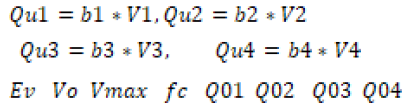
Figure 2 highlights the scheme of the former module of the total model. In it, a set of several reservoirs disposed both in series and parallel transforms the total rainfall and observed temperature data into the corresponding calculated stream flows. Therefore, the total model relies on 11 parameters in total in the modules 1 and 2. The former four (b1, b2, b3, b4) are related to the so-known state equation (1) of each reservoir:

Figure 2: Scheme of the adopted reservoirs.
 (1)
(1)
while V0 and Vmax correspond, respectively, to the initial value and maximum value of the first reservoir, fc is the infiltration capacity of soil and Q01, Q02, Q03, Q04 correspond to the initial stream flow values of the remaining reservoirs.
Data description
Sub hourly rainfall, temperature and level data are available for 39 catchments in the North-Eastern side of Italy, in Liguria Region located next to French border. Each datum is observed every fifteen minutes and the final value is recorded. For instance, if we deal with water level (model’s target output), a given record is not the average value occurred over the fifteen minutes time interval but the last punctual value at the end of the interval itself. Same can be said for rainfall and temperature.
Almost all the 39 and in particular the 10 catchments under study are characterized by similar hydrological response having intensive rainfall mostly during April and November with sudden flash floods with time concentration of the order of a couple of hours. According to Table 1, catchments number: 2,4,5,6 and 9 have also historical rating curves since they were historically monitored catchments recently restored. Overall yearly cumulative rainfall for each catchment overtakes 1.2 m.
| Station number | River | Gauging station |
|---|---|---|
| 1 | Armea | Valle Armea |
| 2 | Argentina a |
Merelli |
| 3 | Argentina a |
Montalto |
| 4 | Arroscia | Ortovero |
| 5 | Neva | Cisano |
| 6 | Bisagno | La Presa |
| 7 | Aveto | Cabanne |
| 8 | Sturla | Vignolo |
| 9 | Vara | Nasceto |
| 10 | Vara | Brugnato |
Table 1: List of study area.
The city of Genova and western basins (Right side of Figure 3) can show cumulative precipitation up to 2 m/year. The city of Genova is notorious for experiencing flooding of its two rivers, Bisagno and Fereggiano, which have the last 40% of their total length subterranean before they reach the sea. When these rivers reach the urbanized area of Genova and become subterranean, they can become pressurized very quickly, lifting up manholes and superficial covers. After the flood of November 2011 during which in less than 5 hours more than 600 mm have fallen causing deaths of 20 people in the hit area, two expansion boxes have been designed to allow urban rivers to laminate properly.
The rating curves have been cut into three parts: low, middle and high part. The lower part goes from almost null stream flow up to 2 m3/s (which corresponds roughly to rivers wade across conditions), the middle part reaches up to 50 m3/s and the last part till high floods up to 300-400 m3/s.
For Genova and the western basin, evaluation of highest part of the rating curve is more useful in order to give proper alerts for flash floods. However, for the eastern basins, water management and availability, and therefore, the lower part of the rating curve gives more practical results for the operation of hydropower installations.
Figure 3 reports the location under study and shows the study catchments. The total level data set covers an area of approximately 5400 km2. Therefore, the instrumental density corresponds to 5.35 gauges per km2. A case in point level registrations has inherited 19 historical instruments displaced near the catchments’ deltas and new additional instruments located in the upper part of the basins. The historical hydrometers have been allocated for water availability purposes next to catchments deltas, and their corresponding daily stream flows have been published roughly regularly from 1930 till 1977. Conversely, the additional new 21 hydrometers have been used to give responses to public alert against sudden and explosive flash floods due to the worsen after 1970s by sudden and chaotic increase after 1970. Still, starting from the period during which new hydrometers have been installed (in the beginning 2000) neither the stream flow sequence nor the rating curve is available for any above-mentioned catchment at any time scale.

Figure 3: Map of the Liguria region.
The modelling procedure has been carried out having considered a unique rainfall and temperature station of reference for each catchment. The station is located approximately barycentre to the basin. More in details: it may occur that either a unique registration instrument is already at disposal and displaced in a roughly barycentre place; or, conversely, the information is reported to the barycentre from nearby rainfall gauges having introduced the inverse of the square distance between each instrument and the barycentre itself.
In reference to the thermo metrical information the lack in data has been integrated relying on nearby stations relying on the gradient method. At last, in case a considerable amount of collected data is missing (i.e., a couple of months); the entire modelling has been deserted for that specific catchment under study.
Other physical variables, typically linked to the topographic information, have been disregarded since the model works in a lumped way. Data records, for each station, vary in length starting from two years of information (for very recent stations) up to 15 years having longer records for the historically installed hydrometers. Interpolation of input data, despite its related uncertainties, has revealed to be necessary because totally unbroken records are not at disposal (Figures 4-6).

Figure 4: Monthly average values: total sequences.

Figure 5: Monthly average values: Effective rainfalls sequences.

Figure 6: Monthly average values: stream flow sequences.
Shape of flow duration curve
Following [9] “The flow duration curve is a cumulative frequency curve that shows the percent of time specified discharges were equaled or exceeded during a given period. It combines in one curve the flow characteristics of a stream throughout the range of discharge without regard to the sequence of occurrence”. Moreover, as reported by [10], the two most important characteristics about stream flow duration curves are the runoff coefficient and the shape of the curve. In order to focus on the shape of the curves, Flow Duration Curves, namely, FDCs can be expressed as daily, weekly and monthly flow data are graphed in Figures 7-9 for the ten catchments under study. Flows have always been normalized by their mean values to allow comparisons.
All curves show very flat tails. Conversely, the upper parts of the curves highlight the intermittent flow regime of these rivers thus having the monthly curve (Figure 9) differing considerably from the daily curve (Figure 7). The shape of the curve is determined by the hydrologic and geologic characteristics of the drainage area. Referring to daily stream flow curves (Figure 7) which have been used almost exclusively in recent studies [3,5], the flat slope reveals the presence of surface and ground water storage which tends to equalize the flow. In a nutshell, the flat slope indicates a large amount of water storage for all catchments.

Figure 7: Flow duration curves at daily scale.

Figure 8: Flow duration curves at weekly scale.

Figure 9: Flow duration curves at monthly scale.
Runoff coefficient: Procedure description
Figures 10 and 11 report the comparison between historical and modelled rating curves. For sake of synthesis only the results for Arroscia river are shown.

Figure 10: Historical rating curve.

Figure 11: Modelled rating curve.
The modelled curve diverges slightly to the past 1975 curve, which is considered the target curve of reference. Therefore, a constraint on the modelling procedure needs to be introduced. Runoff constraint is considered to be the ratio between the long-term annual runoff vs. the long-term annual precipitation. The global model has been once again recalibrated having introduced a constraint on the second module. In this case, having noticed that the ideal value for the runoff coefficient (R) reaches 0.7, the bounds of condition inside which R lies are set between 0.65-0.75.
There is a big change late in 2014 in November that leads to change in the corresponding rating curves. For instance, at the end of 2014, 50.2 mm occurred in one hour. This period corresponds roughly to November the 3rd. Generally, in November and April high rainfall occurs. In order to better investigate how data can affect model’s performance, a longer database of calibration ought to be considered. Entire data set for Arroscia rivers, covers the period of 2003-2017. So, as completeness to Figure 13, the total level series is plotted in Figures 12-15.

Figure 12: Historical level series 2003-2005.

Figure 13: Historical level series 2012-2017.

Figure 14: Historical level series 2009-2011.

Figure 15: Historical level series 2006-2008.
Sensitivity Analysis
Sensitivity analysis reveals how the uncertainty in the output of a mathematical model is related to different sources of uncertainty in the inputs. Generally speaking, a mathematical model can be highly complex, and, as a result, its relationship between input and output may be poorly understood. In such a case, the model can be considered a black-box approach, having the output a consequence of its inputs with no detail on the physical process under study. Good modelling requires a modeller to provide not only the results but, mostly, the evaluation of the confidence in the model. This requires a quantification of the uncertainty in any model result (alternatively known as uncertainty analysis) and second, an evaluation of how much each input contributes to the output uncertainty. Sensitivity analysis is related to the second of this issue performing the role of ordering the strength and relevance of the inputs determining the variation in the output. Several approaches of sensitivity analysis can be carried out such as: computational expense, correlated inputs, model interaction, multiple outputs. The reader is sent back to the corresponding literature for details. Herein the One at Time (OAT/OFAT) approach is adopted in order to discover how the method affects model outputs. This is also known as OAT. The procedure consists of two steps
1) Returning the variable in its nominal value, then
2) Repeating for each of the other inputs in the same way
Sensitivity may be then measured by monitoring changes in the output as partial derivatives or linear regression. This appears a logical approach as any changed observed in the output will be unambiguously be due to the single variable changed. Moreover, by changing one variable at a time, one can keep all other variables fixed to the central values. This method is generally preferred because of its practical reasons.
Sensitivity Analysis: Arroscia River 2014
The reader is sent back to [11-19] for further details. The procedure has been adopted to Arroscia River. The model has been run using data of 2004. As expressed above, at first a 10% amount has been added to each selected parameter. Table 2 shows the obtained results while reporting:
|
Tri/par r |
Initial values | #1 | #2 | #3 | #4 | #5 | #6 | #7 | #8 | #9 | #10 | #11 |
|---|---|---|---|---|---|---|---|---|---|---|---|---|
| 1/a1 | 6.122 | 6.631 | Id | Id | Id | Id | Id | Id | Id | Id | Id | Id |
| 2/b1 | 1.97E-02 | id | 5.7E-3 | id | Id | Id | Id | Id | Id | Id | Id | Id |
| 3/c1 | 1.6826 | id | id | 1.5793 | Id | Id | Id | Id | Id | Id | Id | Id |
| 4/b2 | 0.1585 | id | id | Id | 0.17099 | Id | Id | Id | Id | Id | Id | Id |
| 5/c2 | 2.588 | id | id | Id | Id | 2.6513 | Id | Id | Id | Id | Id | Id |
| 6/ y11 | 0.4388 | id | id | Id | Id | Id | 0.425 | Id | Id | Id | Id | Id |
| 7/y12 | 1.4674 | id | id | Id | Id | Id | Id | 1.593 | Id | Id | Id | Id |
| 8/b3 | 6.388E-02 | id | id | Id | Id | Id | Id | Id | 0.2976 | Id | Id | Id |
| 9/c3 | 1.3785 | id | id | id | Id | Id | Id | Id | Id | Id | Id | |
| 10/y13 | 2.98 | id | id | Id | Id | Id | Id | Id | Id | Id | 2.96 | Id |
| 11/b4 | 2.9516 | id | id | id | Id | Id | Id | Id | Id | Id | Id | 2.97 |
Table 2: Results with sensitivity analysis.
• In the first column the initial values of the parameters are reported.
• From column #1 to column #11 a 10% is added to each parameter, as the row changes item
• Id stands for identical meaning that the parameter has been considered fixed to its initial
• Value for the selected trial #.
Comments
In this work, flow duration curve and stream flow sequences have been provided for ten catchments located in the north western side of Italy for 2014. Starting from a scenario of only hydrometric levels available with no corresponding flows, the study shows a method to supply flows adopting a lumped conceptual model based upon 11 parameters. The model is poorly demanding in input data as it requires only rainfall and temperature data. This can be an advantage toward synthetically monitored catchments. The approach introduced in this paper provides a prediction for small catchments characterized by intermittent and torrential flow regime. A detail on historical (1970) flow duration curves has also proved a common behavior of the area having the hydrological year beginning at the middle of August and prolonged low flows at the end of August/beginning of September. Catchments with a small area, high elevation and high slope are demonstrated to respond to a rainfall event with a sudden peak in stream flow that accounts for most of the incident rainfall. This is mainly the reason why R may be higher for those catchments respect to larger ones. A powerful use of the Runoff Coefficient in regionalization of rainfall runoff models has been introduced by Croke et al. [10] and herein considered. For the sake of simplicity results related only to Arroscia river are reported. At the end, in order to provide a good modelling, sensitivity analysis is also introduced. Good modelling, in fact, means that a modeller provides not only the results but, mostly, the evaluation of the confidence in the model. Further developments of the procedure with focus on stream flow duration curve parameters constraints and application on NSW water courses are favourably recommended [20-29].
References
- WMO (2010) Manuals on Stream Gauging WMO- No. 1044, ISBN 978-92-63-11044-2.
- Horner I, Renard B, Le Coz J, Branger F, Mcmillian H, et al. (2018) Impact of stage measurement errors on stream flow uncertainty. Water Resour Res 54:1952-1976.
- Bartolini P, Mondino M, Carcano E (2016) Determinazione delle scale di deflusso con un metodo misto idrologico idraulico.
- Morlot T, Perret C, Favre AC, Jalbert J (2014) Dynamic Rating curve assessment for hydrometric stations and computation of the associated uncertainty quality and station management indicators. J Hydrol 517:173-186.
- Morrison DA, Kingwell RS, Pannell DJ. Ewing MA (1986) A mathematical programming model of a crop livestock farm system. Agric Syst 20:243-268.
- Ball JE, Kerr A, Rocha GC, Islam, A (2016) A review of stream gauge records for design flood estimation, Proc.37th Hydrology and Water Resources Symposium: Water, Infrastructure and the Environment, Â HWRS , Queenstown, NZ.
- Fenton JD, Keller RJ (2001) The calculation of stream flow from measurements of stage, Technical Report 01/6, September. Cooperative Research Centre for Catchment Hydrology.
- Todini E (1998) Rainfall runoff modeling - Past present and future. J Hydrol 100:341-352.
- Searcy JK (1959) Flow duration curve Manual of hydrology Part 2, Low flow tecniques. Geological Survey Water Supply Paper 1542.
- Croke B, Norton JP (2004) Regionalization of rainfall runoff models, Conference: 2nd Biennial Meeting of the International Environmental Modelling and Software Society at Osnabruck, Germany.
- Hamby DM (1995) A comparison of sensitivity analysis techniques. Health Phys 68:195 -204.
- Annali Idrologici (1952-1977) Â Ministero dei Lavori Pubblici, Servizio Idrografico, sezione autonoma del genio civile con sede di Genova, bacini con foce del litorale tirrenico, dal Roja al Magra, Roma, Istituto Poligrafico dello Stato.
- Clemson B, Tang Y, Pyne J, Unal R (1995) Efficient methods for sensitivity analyisis. Syst Dyn Rev 11: 31-49.
- Fernandez W, Vogel RM, Sankarasubramanian A (2000) Regional calibration of watershed model. Hydrol Sci J 45: 689-707.
- Hamby DM (1994) A review of techniques for parameter sensitivity analysis of environmental models. Environ Monit Assess 32:135-154.
- Hallam D (1987) MIDAS a bioeconomic model of a dryland farm system: Kingwell, R. S. and Pannell, D. J. (Eds). Pudoc, Wageningen. Agric Syst 26:164-163.
- Kottegoda NT, Rosso R (1997) Statistics, probability and reliability for civil and environmental engineers, MacGraw Hill, New York, USA.
- Mckay MD (1995) Evaluating prediction uncertainty. Los Alamos National Laboratory, Neureg /CR 6311 (LA 12915 MS).
- MacMahon T, Murray C, Peel, (2019) Uncertainty in stage -discharge rating curves, Application to Australia Hydrologic Reference Stations data. Hydrol Sci J 64:255 275.
- Norblom TL, Pannell DJ (1994) From weed to wealth? Prospects for medic pastures in mediterranean farming system of northwest Syria. Agric Econ 11: 29-42
- Insua RD (1990) Sensitivity analysis in multi objective decision making. Lecture notes in economics and mathematical systems. 347.
- Seibert J (1999) Regionalization of parameters for a conceptual rainfall runoff model. Agric For Meteorol 98: 279-293.
- Spate JM, Croke BFW, Norton JP (2004) A proposed rule-discovery scheme for regionalization of rainfall runoff characteristics in New South Wales, Australia. In transaction of the 2nd biennial meeting of the international environmental modeling and software society, iEMS Manno, Switzerland, Â ISBN 88-900787-pp 1-5.
- Sudheer KP, Jain SK (2003) Radial basis function neural network for modeling rating curves. JÂ Â Â Â Â Â Â Â Â Â Â Â Â Â Hydrol Eng 8:161-164.
- Uyeno D (1992) Monte carlo simulation on micro computers simulation. 58: 418-423.
- Vrugt JA, Gupta HV, Bouten W, Sooroshian SA (2003) A shuffled complex evolution metropolis algorithm for optimization and uncertainty assessment of hydrologic model parameters. Water Resour Res 39:1201
- Wagener T, Boyle D, Lees MJ, Wheater HS, Gupta HV, Sooroshian S (2001) A framework for the development and application of hydrological models. Hydrol Earth Syst Sci 5: 13-26.
- Yadav M, Wagener T, Gupta H (2007) Regionalization of constraints on expected watershed response behavior for improved predictions in ungauged basins. Adv Water Resour 30: pp. 1756-1774.
- Yu PS, Yang TC (2000) Using synthetic flow duration curves for rainfall runoff model calibration at ungauged sites. Hydrol Process 14: 117- 133.
Citation: Carcano E (2021) A Procedure to Assess Stream Flow Rating Curves and Stream Flow Sequences. Innov Ener Res, 10: 257.
Copyright: © 2021 Carcano E. This is an open-access article distributed under the terms of the Creative Commons Attribution License, which permits unrestricted use, distribution, and reproduction in any medium, provided the original author and source are credited.
Select your language of interest to view the total content in your interested language
Share This Article
Recommended Journals
Open Access Journals
Article Usage
- Total views: 2698
- [From(publication date): 0-2021 - Dec 19, 2025]
- Breakdown by view type
- HTML page views: 2029
- PDF downloads: 669