Adaptive Comfort Model Incorporating Temperature Gradient for a UK Residential Building
Received: 03-Apr-2019 / Accepted Date: 11-Apr-2019 / Published Date: 17-Apr-2019 DOI: 10.4172/2168-9717.1000227
Abstract
Thermal comfort field experiments were conducted to acquire thermal comfort data of 119 participants in a test house representative of a typical UK house. This paper compares the performance of popular PMV-based thermal comfort index vs neutral temperature based on Actual Mean Vote. The aim of this research was to incorporate vertical thermal gradient, which is usually a neglected yet highly influential parameter in a residential setting and propose a new adaptive thermal comfort model. The new adaptive model (LPMV) has been developed using a polynomial curve fit method. This method was chosen as it has the capability to correlate indoor environmental parameters with AMV and incorporated them in the generated mathematical model. The model requires temperature gradient and SET* only to determine neutral temperatures which makes it the first of its kind. The LMPV model was rigorously tested against thermal comfort data compiled in this study and against independent/unbiased data (the ASHRAE RP-884 database). LPMV showed up to 0.7°C improvement in predicting neutral temperature of occupants compared to the famous Fanger’s PMV model. This can result in better prediction of a suitable heating setpoint temperature which has great implications on annual energy demand.
Keywords: Thermal comfort; Building physic; Temperature gradient; Fanger; AMV; PMV
Abbreviations
AMV: Actual Mean Vote; PMV: Predicted Mean Vote; LPMV: Loughborough PMV model; SET: Standard Effective Temperature
Nomenclature
ta: Air Temperature;
td: Dew-Point Temperature;
T0.6: Air Temperature at 0.6 m from the floor;
TG: Temperature Gradient i.e. temperature difference between 0.1 m and 1.1 m above the floor.
Introduction
The thermal comfort sensation of occupants in an indoor environment is dependent on the environmental conditions (air temperature, mean radiant temperature, operative temperature, air speed, absolute humidity) as well as their metabolic rate and clothing insulation. Fanger’s comfort model known as Predicted Mean Vote (PMV) is typically used by researchers and practitioners in predicting occupant’s thermal comfort. Fanger’s PMV model assumed that thermal sensation is a function of the thermal load on the body and highlighted the associations using a mathematical model. This model was based on a survey of thermal sensation surveys collected from participants in a climate chamber. However, thermal comfort tests conducted in countries around the world show a variation in the accuracy of the PMV model in predicting occupant thermal comfort for both test chamber and field studies [1-4]. It has been advised that thermal comfort models need to be researched that are specifically applicable to a certain geographical location and climate. This encourages the investigation of a modified PMV model that is more accurate in predicting thermal comfort of European participants in a European winter climate.
After Fanger’s PMV model, Gonzalez and Gagge proposed a twonode model that was suitable for a specific range of indoor air humidity and velocity known as Standard Effective Temperature (SET*) which is a subset of new Effective Temperature (ET*) under standardised condition in a sedentary activity [5]. ET* is defined as the dry bulb temperature (DTB) of uniform enclosure with 50% relative humidity at sea level [5]. After the addition of PMV into the ASHRAE and ISO 7730 standards in the early 1980s, Gagge et al. [1] improved the PMV model by incorporating ET* and SET* (Standard Effective Temperature) into the PMV formula and is known as PMV* [1]. Most of these studies were conducted in an environment chamber with seated participants doing sedentary activities with an assumed metabolic rate of 1.0 met.
Although Fanger’s model was accepted as an international standard, the limitation of the application of the PMV model for practical nonair conditioning building has resulted in the development of different PMV variations. For example, for hot and humid climate ePMV was developed by Fanger and Toftum [2], aPMV developed by Yao et al. using black box modelling for Chinese participants and PMVn [3,6]. As these models were developed for different climates and cultures their suitability for UK residential buildings needs further investigation.
Humphreys and Nicol argued that the PMV model’s success was due to the model being applied in air-conditioned buildings with narrow ranges of operative temperature [7]. They then developed a new thermal comfort model, based on the multiple regression analysis of the ASHRAE RRP-884 dataset with more dynamic ranges of indoor temperature. Zhang et al. conducted a human local discomfort study in a stratified environment by using a controlled environmental chamber with 109 participants which later developed the CBE comfort model [8].
Yao et al. explored adaptive comfort with 3D curve fit method on PMV data [3]. Gao et al. developed eTSV and modified SET* model based on his dataset by using aPMV and ePMV methods [9]. This research distinguished the methods by air speeds of less than and more than 0.2 m/s. Gao et al. also found that the modified SET* had better accuracy in predicting the reported thermal sensation (TSV) compared to the modified PMV [9].
The performance of each of these models needs to be verified in predicting thermal comfort with the help of distinct databases. Thus, in this study the suitability of PMV-based models such as Fanger’s PMV, Gagge Pierce two-node: SET* and new effective temperature ET* models were evaluated in a test house. Little research has been conducted in residential buildings with a large set of participants thus the aim is to use a large number of participants as test subjects. Additionally, as residential buildings with smaller volumes and radiator heating are more prone to sharp gradients in vertical air temperatures (temperature gradients). This is because of smaller volumes with 0.87 ACH may contribute to uneven air temperature during winter as a lower air change rate will reduce vertical air stratification [10].
In this paper, a new comfort model has been developed that incorporates temperature gradient of the space in predicting suitable temperatures for occupants. This was possible using the polynomial plot method [6]. In this method a 3D curve fit is plotted between three influential parameters to define the neutral temperature of the participants. This is different to linear fits that are plotted between two influential parameters. This method was chosen as it has the capability to correlate a second indoor environmental parameter with AMV [11].
Methodology
The test house
Thermal comfort tests were conducted from October to November of 2015 and November to December of 2016 in a two-storey detached test house with exposed mass located in the Midlands (Figure 1). The test house located in the Holywell Park of the Loughborough University campus is a North-West facing, two storey residential detached building with a pitched roof. The exterior of the test house is exposed brick work and was built in the 1998. It consists of 2 bedrooms, 1 kitchen, 1 living room, 1 toilet and 1 bathroom. The test house has a heat loss coefficient of 136 W/K and an infiltration rate of 0.87 ach measured in 3 consecutive seasons by Jack R. The infiltration rate was measured using a blow door test and is relatively high compared to an average of 0.4 each for a UK home. The house is classified as medium air tightness and is moderately insulated according to BSI-13790 [12]. All the comfort surveys and tests were carried out in the living room the dimensions of which are presented in Table 1.

Figure 1: Exterior isometric view of the test house.
| Description | Area |
|---|---|
| Floor to ceiling height | 2.35 m |
| Floor area | 16.66 m2 |
| Door area | 1.68 m2 |
| Windows area | 4.49 m2 |
Table 1: Dimensions of the living room.
Experimental procedure
A total of 119 students (both male and female) took part in the thermal comfort experiments. On average four subjects were present at each thermal comfort session. Participants from outside the house were then introduced into the kitchen area where they were explained the procedure of the experiments and asked to sign a consent form. The 30 min buffer in the kitchen was also created so that the participants became thermal neutral with the environment, meaning external weather affects became minimal. They were then taken to the living room where they were asked to take a seat on the sofas and carry out work such as reading or watching TV/tablet. The four subjects were allowed for any adaptive opportunities such as changing their clothing levels, opening a window or tempering with the heating system throughout the duration of the test sessions. The participants were asked to answer questionnaires at 0, 15, 30, 45 …. 120 minutes mark. For the same 15 minutes intervals readings were taken from the sensors and PMV was calculated. A total of 54 sessions of thermal comfort survey with different subjects were conducted and 1837 datasets were collected.
Sensor measurements consisted of 4 environmental indoor parameters (air temperature, mean radiant temperature, air velocity and relative humidity). These were measured by the thermal comfort kit (Figure 2a and 2b) with the detail specifications in Table 2. The operative temperature was measured via sensor whilst Tmrt was calculated using eqn. (1). The thermal comfort kit was placed in front of participants with a distance greater than 30 cm away from the subjects and at a height of 60 cm from the floor in the living room [13]. A data logger was used to measure the outdoor air temperature together with the air temperature stratification inside the room at heights of 0.1 m, 0.6 m, 1.1 m and 1.7 m from the floor. The participants were observed for their clothing levels and the activities they were conducting. These were then reference with CIBSE guide A to calculate an average clo value with the sofa resistivity of 0.76 clo with a tolerance of ± 0.04 and the sedentary metabolic rate of 1.0 met which is equivalent to 58.2 W/m2.

Figure 2: (a) Typical setup of participants filling in surveys (b) Thermal comfort kit for the indoor environment surveys.
| Instruments | Description | Range | Accuracy |
|---|---|---|---|
| Lumisense INNOVA 1221 Thermal comfort controller | Thermal comfort controller | N/A | ±0.1°C |
| Operative temperature Model number: MM0060 | Read indoor operative temperature | 5-40°C | ±0.3°C |
| Air temperatureModel number: MM0034 | Read indoor air temperature | 5-40°C | ±0.2°C |
| Relative Humidity Model number: MM0037 | Read relative humidity, Dew bulb temperature | -20 to 50°C with Operating temperature: 5-40°C | ta-td < 10 K: ±0.5 K or ±0.05 kPa 10 K < ta-td <25 K: ±1.0 K or ±0.1 kPa |
| Air speed Model number: MM0038 | Air velocity sensor | 0 to 10 m/s | ±0.05 m/s |
| Air Temperature Thermistor NTC U Type | Air temperature sensor for temperature gradients | -50 to 70°C | Accuracy of ±0.2°C |
| Onset HOBO U8-001-08 | Air temperature sensor | -20° to 70°C | Accuracy of ±0.47°C |
Table 2: Dimensions of the living room.
Tmrt=(Top x 2)-Ta (1)
The survey measurements were based on the 7-point Bedford comfort scale and ASHRAE Standard 55 questionnaire on thermal sensation [14]. The participants were asked to report their thermal sensation (TSV/AMV) between -3 to 3 every 15 minutes. This may seem short time duration for the human body to adapt but skin sensation does adapt quickly. Another reason this time duration was chosen is because it is what past researchers have also utilised [15].
Performance Analysis of Current PMV Based Models
Before a new comfort model is generated for the current experimental data it was important to see which of the currently established comfort models perform the best in predicting thermal comfort of the participants. To conduct the performance analysis of the various comfort models a datum parameter was selected. For this study it was the neutral temperature (Tn) which is the temperature at which participants would feel the most comfortable with their thermal environment. Tn is calculated using the linear regression method on the AMV data points versus operative temperature (Top). The following PMV based models were chosen as the candidates:
ePMV=e × PMV (Fanger and Toftum) [2]
aPMV=PMV/(1+λ * PMV) (Yao et al.) [3]
PMVnew=0.8(PMV − Dpmv − vote) (Nicol and Humphreys) [7]
PMVn=−5.151+0.202Ta+0.553Vp (Orosa) [7]
TSVse=ePTS (Gao et al.) [9]
TSVsa=PTS/(1+λPTS) (Gao et al.) [9]
PMVashrae=−6.802+0.243Ta+0.278Vp (ASHRAE) [6]
PMVSET∗ =(0.028+0.303e−0.036M) × (H − Lset) (Gagge) [1]
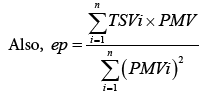
ePMVgao=ep × PMV (Gao et al.) [9]
Please note: H is the internal heat production rate per unit area (W/ m2). L represents all modes of energy loss from body (W/m2) in PMV. SET* will replace Top in PMV to become PMVSET*.
The neutral temperature based on the AMV of all the occupants was determined using linear regression to be 23.4°C. This is higher than the recommended temperature range of 22-23°C by CIBSE for living rooms in a residential property [16]. It was interesting to understand how the different comfort models stated previously perform in predicting this neutral temperature. Fanger’s famous PMV model predicted a neutral temperature of 24.2°C which results in a standard deviation (SD) of 0.8°C which is illustrated by red bars in Figure 3. In the same figure, SD from utilising other adaptive models is illustrated using blue bars. It can be observed that TSVse and ePMVgao perform the best with an SD of 0.78°C and followed closely by ePMV with a SD of 0.79°C [17-19].

Figure 3: Standard deviation of different adaptive comfort models in predicting neutral temperature based on AMV.
Incorporating Temperature Gradient
Temperature gradient (TG) in these experiments refers to the air temperature gradient between two points i.e. 0.1 m and 1.1 m above the floor. In this study, a temperature gradient of up to 7.3°C was measured. The average AMV during the study elucidated that participants accepted higher TG with ± 0.5 votes. How do you know if it was acceptable??? It was accepted due to based on Pearson’s statistical correlation and significance carried out on the experimental data is was found that TG shows a strong correlation with AMV thus it was decided to incorporate the parameter into the comfort model using the curve fit approach used by Orosa and Oliveira and investigate its performance [11]. The curve fit approach consisted of plotting a 3D curve fit between three influential parameters to better predict occupant comfort (Figures 4-8). This method was conducted for numerous combinations of three influential parameters. Five of the best performing models are the following:

Figure 4: LPMV1 3D curve fit between AMV, TG and TSVsa.

Figure 5: LPMV2 3D curve fit between AMV, TG and ePMV.

Figure 6: LPMV3 3D curve fit between PMV, TG and SET.

Figure 7: LPMV4 3D curve fit between PMV, TG and Top.

Figure 8: LPMV4 3D curve fit between AMV, TG and PMV.
LPMV1=−0.294 − 0.02402 × TSVsa+0.13 × TG; TSVsa=(PTS/ (1+λPTS)),
where, the adaptive coefficient λ was obtained based on the equation used by Yao and found to be 0.235. The PTS was equal to 0.1185 × SET − 2.7775 using Gao, et al. method [9].
LPMV2=−0.2864+0.08308 × e(PMV) +0.1308 × TG; e=0.8

LPMV5=−0.2402+0.3126 × PMV+0.1289 × TG
The SD of the stated five LPMVs (Loughborough PMVs) and some other combination of influential parameters is presented in Figure 9. The SD of all the 3D curve fit based models (blue bars) is less than Fanger’s PMV model (shown in red dotted line). It can also be seen that the five models LPMV1 to LPMV5 have significantly less SD in predicting occupant’s neutral temperature.

Figure 9: Standard deviation of 3D curve fit based PMV models in predicting neutral temperature compared to Fanger's PMV.
In order to conduct scientific rigour, the five LMPV models will be tested against unrelated thermal comfort data that was compiled from different experiments by other researchers in different locations in the UK. For this reason, data from the RP-884 database in South Wales and Liverpool, UK have been utilised. Figure 10 presents the comparison between the different comfort models against the Fanger’s PMV model. Some of the five selected models do perform better than PMV for either South Wales or Liverpool’s data. However, LPMV3 is observed to perform better than Fanger’s PMV in predicting neutral temperature for both data sets. LPMV3 exhibited and improved SD of 0.1°C for the South Wales data whilst an improved SD of 0.7°C for the Liverpool data. This is a significant improvement in neutral temperature prediction and can have consequences in terms of energy use when specifying heating setpoint temperature.

Figure 10: Performance analysis of different comfort models in predicting neutral temperatures from the Rp-884 database in South Wales and Liverpool, UK.
Results and Conclusions
This paper presents the development of an improved mathematical model that can predict occupant thermal comfort in a residential building (specifically in a living room area). The method employed is of plotting polynomial fit curves between the most influential parameters that affect AMV. The aim was to incorporate temperature gradient, a parameter that is usually ignored in generating comfort models. The best performing LPMV model utilises both vertical temperature gradient, TG and SET for predicting thermal comfort. It was observed that LPMV model had a SD of 0.76 compared to Fanger’s PMV model of 0.83 in predicting neutral temperatures of occupants participating in this study. This difference might not be significant in this specific test scenario, but the improved model does promise better performance which might be amplified in other applications. Furthermore, the LPMV model was observed to better predict neutral temperature (0.2°C cooler) compared to Fanger’s PMV model for independent thermal comfort data (RP-884 database). It needs to be noted here that this model performed better than Fanger’s model for test case with high temperature gradients whilst PMV is more suited for uniform conditions. Thus, the application of LMPV is more suited for areas where high temperature gradients are expected. This can have immense effect in choosing set point temperature of the heating system and consequently the energy use. This model is recommended for use in residential houses with strong temperature gradients such as the rooms heated by radiators which are common in UK houses.
References
- Gagge AP, Fobelets A, Berglund I (1986) A standard predictive index of human response to the thermal environment. ASHRAE Trans (United States) 92.
- Fanger PO, Toftum J (2002) Extension of the PMV model to non-air-conditioned buildings in warm climates. Energy and Buildings 34: 533-536.
- Yao R, Li B, Liu J (2009) A theoretical adaptive model of thermal comfort-Adaptive Predicted Mean Vote (aPMV). Building and Environment 44: 2089-2096.
- Standard A (2004) Standard 55-2004. Thermal environmental conditions for human occupancy, pp: 9-11.
- Gonzalez R, Nishi Y, Gagge A (1974) Experimental evaluation of standard effective temperature a new biometeorological index of man's thermal discomfort. International journal of biometeorology 18: 1-15.
- Ashrae A (2004) Standard 55-2004. Thermal environmental conditions for human occupancy, 744.
- Humphreys MA, Nicol JF (2002) The validity of ISO-PMV for predicting comfort votes in every-day thermal environments. Energy and Buildings 34: 667-684 OROSA.
- Zhang H (2003) Human thermal sensation and comfort in transient and non-uniform thermal environments.
- Gao J, Wang Y, Wargocki P (2015) Comparative analysis of modified PMV models and SET models to predict human thermal sensation in naturally ventilated buildings. Building and Environment, 92: 200-208.
- Hongtao X, Gao N and Niu J (2008) The method to quantifying the supply airflow rate in the under-floor air distribution (UFAD) systems. Indoor Air, 17-22.
- Jose A, Oliveria AC (2011) A new thermal comfort approach comparing adaptive and PMV models. Renewable Energy, 36: 951-956.
- BSI 2008. ISO 13790. Energy performance of buildings. Calculation of energy use for space heating and cooling.
- Beizaee A, Firth SK, Vadodaria K, Loveday DL (2012) Assessing the ability of PMV model in predicting thermal sensation in naturally ventilated buildings in UK.
- Goto T, Toftum J, De Dear R, Fanger PO (2006) Thermal sensation and thermophysiological responses to metabolic step-changes. International journal of biometeorology 50: 323-332.
- CIBSE (2006) Environmental Design (CIBSE Guide), Chartered Institution of Building Services Engineers; 7th Revised edition edition.
- Bedford T (1936) The Warmth Factor on Comfort at Work. Rep. Industr Health Res Boad, 76.
- Fanger PO (1970) Thermal comfort. Analysis and applications in environmental engineering. Thermal comfort. Analysis and applications in environmental engineering.
- Zhang H, Huizenga C, Arens EA, YU T (2005) Modeling thermal comfort in stratified environments.
Citation: Samsuddin S, Durrani F, Eftekhari M (2019) Adaptive Comfort Model Incorporating Temperature Gradient for a UK Residential Building. J Archit Eng Tech 8: 227. DOI: 10.4172/2168-9717.1000227
Copyright: © 2019 Samsuddin S, et al. This is an open-access article distributed under the terms of the Creative Commons Attribution License, which permits unrestricted use, distribution, and reproduction in any medium, provided the original author and source are credited.
Select your language of interest to view the total content in your interested language
Share This Article
Recommended Journals
Open Access Journals
Article Tools
Article Usage
- Total views: 4081
- [From(publication date): 0-2019 - Nov 17, 2025]
- Breakdown by view type
- HTML page views: 3170
- PDF downloads: 911