Analytical and Numerical Study to Nonlinear Heat Transfer Equation in Strait Fin
Received: 22-Oct-2016 / Accepted Date: 07-Dec-2016 / Published Date: 13-Dec-2016
Abstract
Akbari-Ganji’s Method (AGM) to study an unsteady nonlinear convective-radiative equation and a nonlinear convective-radiative-conduction equation containing two small parameters of ε1 and ε2 and evaluate the efficiency of straight fins. The concept of Akbari-Ganji’s Method is briefly introduced and employed to derive solution of nonlinear equation. The obtained results from AGM are compared with those of obtained from Homotopy Perturbation Method (HPM), the fourth-order Runge-Kutta Numerical Method (NUM) and FlexPDE software to verify the accuracy of the proposed method. Results show by increasing N efficiency decline. In contrast to, with increasing of ε1, ε2 the value of efficiency increases. In addition to, this study shows that AGM is powerful method to solve nonlinear differential equations, such as the problem raised in this research.
Keywords: Heat transfer; Homotopy Perturbation Method; Akbari- Ganji’s Method; FlexPDE software; Nonlinear equation; Strait fin
19168Introduction
Most of scientific phenomena and problems especially in engineering occur nonlinearly. Heat transfer equations in straight surfaces, are one most applicable of them. One of these surfaces is straight fins. Fins are the most effective instrument for increasing the rate of heat transfer. As we know, they increase the area of heat transfer and cause an increase in the transferred heat amount. A full review on this topic is presented by Krause et al. [1]. Fins are widely used in many industrial applications like air conditioning, refrigeration, automobile, chemical processing equipment and electrical chips. Aziz and Hug [2] used the regular perturbation method to obtain a closed form solution for a straight convecting fin by temperature dependent thermal conductivity. Razani and Ahmadi [3] considered circular fins with a nonlinear temperature-dependent thermal conductivity and an arbitrary heat source distribution and obtained the results for the optimum fin design. Yu and Chen [4] assumed that the linear variation of the thermal conductivity and exponential function with the interval of the heat transfer coefficient and then, solved the nonlinear conducting-convecting-radiating heat transfer equation with the differential transformation method. Furthermore, Bouaziz and Aziz [5] introduced a double optimal linearization method (DOLM) to get a simple and accurate solution for the temperature distribution in a straight rectangular convective–radiative fin with temperaturedependent thermal conductivity. Bouaziz et al. [6] presented the efficiency of longitudinal fins with temperature-dependent thermophysical properties. Also, the effects of temperature-dependent thermal conductivity of a moving fin and added radiative component to the surface heat loss have been studied with Aziz and Khani [7]. Ghasemi et al. [8] solved the nonlinear temperature repartition equation in a longitudinal fin with temperature dependent internal heat generation and thermal conductivity using Differential Transformation Method (DTM). Many different methods have recently introduced to solve nonlinear problems such as Optimal Homotopy Analysis Method (OHAM) [9], Homotopy Analysis Method (HAM) [10-12], Homotopy Perturbation Method (HPM) [13-14], Least Square Method (LSM) [15], Differential Transform Method (DTM) [16], Variational Iteration Method (VIM) [17] and Adomian’s Decomposition Method (ADM) [18], many methods are not considered in this study because of brevity. Akbari-Ganji’s Method (AGM) is a new method that be used for investigation of nonlinear problems. A summary of AGM advantages compared to other methods is as below: Boundary conditions are needed in accordance with the order of differential equations in the solution method but when the number of boundary conditions is less than the order of the differential equation, this approach can engender additional new boundary conditions in regard to the own differential equation and its derivatives. Hence, AGM is a powerful method for solving the nonlinear differential equations such as presented equation in this paper. In the present study, we have applied AGM to find the approximate solutions of nonlinear heat transfer equation in a straight fin. The comparison of the results of AGM, Homotopy Perturbation method (HPM), the fourth-order Runge-Kutta numerical Method (NUM) and FlexPDE software results shows excellent complying in solving this nonlinear problem.
Description of the problem
The example to be studied is the one-dimensional heat transfer in a straight fin with the length of L and the cross section area of A and the perimeter of P (Figure 1).The fin surface transfers heat through both convection and radiation. Suppose the temperature of the surrounding air is T0 and the effective sink temperature for the radiative heat transfer is TS. We assume that base temperature of the fin is Tb and there is no heat transfer of the tip of the fin. It is also assumed that the convection heat transfer coefficient h, and the emissivity coefficient of surface, Eg are both constant while conduction coefficient, k, can be variable.

Figure 1: (a) Geometry of a strait fin (b) x-y view.
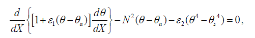
The energy equation and the boundary conditions for the fin are as follows:
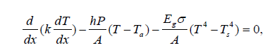 (1)
(1)
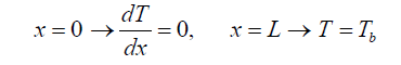 (2)
(2)
Assuming k as a linear function of temperature, we have:
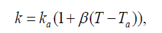 (3)
(3)
After making the equation dimensionless and changing parameters, we have:
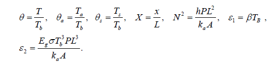 (4)
(4)
And substituting Eq. (6) in Eq. (3) we have:
 (5)
(5)
 (6)
(6)
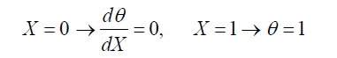
By assuming θa = θs = 0 we have:
 (7)
(7)
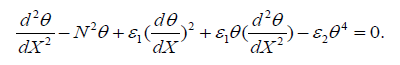
Fin efficiency the heat transfer rate from the fin is found by using Newton’s law of cooling
 (8)
(8)
The ratio of the actual heat transfer from the fin surface to that, that would transfer if the whole fin surface were at the same temperature as the base is commonly called as the fin efficiency
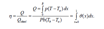 (9)
(9)
Mathematical Procedures
In this section two methods have been examined:
Akbari-Ganji's Method (AGM)
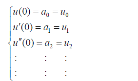
Boundary conditions and initial conditions are needed differential equation according to the physic of the problem. So, we can solve any differential equation with every degrees. In order to comprehend the given method in this research, two differential equations ruling on engineering processes will be solved in this new manner. The nonlinear differential equation of p which is a function of u, the parameter u which is a function of x and their derivatives are considered as follows:
The nonlinear differential equation P (which is a function of u), the parameter u (which is a function of x), and their derivatives are considered as follow:
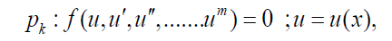 (10)
(10)
Boundary conditions:
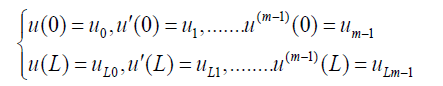 (11)
(11)
To solver the first differential equation, with respect to the boundary conditions in x=L in Eq. (11), the series of letters in the nth order with constant coefficients, which is the answer of the first differential equation, is considered as follows:
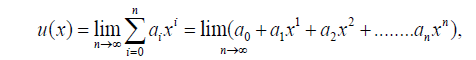 (12)
(12)
The boundary conditions are applied to the function as follows:
a) The application of the boundary conditions for the answer of differential Eq. (12) is in the form of
If x=0
 (13)
(13)
And when x=L
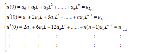 (14)
(14)
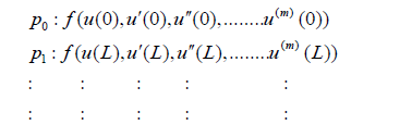
b) After substituting Eq. (14) into Eq. (10), the application of the boundary conditions on differential Eq. (10) is done according to the following procedure:
 (15)
(15)
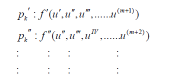
With regard to the choice of n; (n<m) sentences from Eq. (12) and in order to make a set of equations which is consisted of (n+1) equations and (n+1) unknowns, we confront with a number of additional unknowns which are indeed the same coefficients of Eq. (12). Therefore, to remove this problem, we should derive m times from Eq. (10) according to the additional unknowns in the afore-mentioned set differential equations and then this is the time to apply the boundary conditions of Eq. (11) on them.
 (16)
(16)
Application of the boundary conditions on the derivatives of the differential equation Pk in Eq. (16) is done in the form of
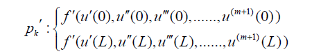 (17)
(17)
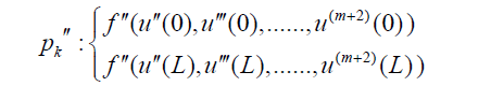 (18)
(18)
The (n+1) equations can be made from Eq. (13) to Eq. (18) so that (n+1) unknown coefficients of Eq. (12) for example a0,a1,a2,a3...an, can be computed. The answer of the nonlinear differential Eq. (10) will be gained by determining coefficients of Eq. (12).
Homotopy Perturbation Method (HPM)
To explain the basic ideas of this method, we consider the following nonlinear differential equation:
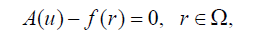 (19)
(19)
With the boundary condition of:
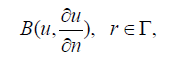 (20)
(20)
Where A is a general differential operator, B a boundary operator, f(r) a known analytical function, ( Γ ) is the boundary of the domain (Ω) and ( ∂u / ∂n ) denotes differentiation along the normal drawn outwards from (Ω).
A can be divided into two parts which are L and N, where L is linear part and N is nonlinear part. Eq. (19) can therefore be rewritten as follows:
 (21)
(21)
Homotopy perturbation structure is shown as follows:
 (22)
(22)
Where,
 (23)
(23)
In Eq. (22), p∈ [0, 1] is an embedding parameter and u0 is the first approximation that satisfies the boundary condition. We can assume that the solution of Eq. (22) can be written as a power series in P, as following:
 (24)
(24)
and the best approximation for solution is:
 (25)
(25)
Application of described methods in the problem
Akbari-Ganji’s Method (AGM)
First of all we rewrite the problem Eq. (7) in the following order:
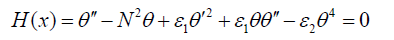 (26)
(26)
In AGM, the answer of the differential equation is considered as a finite series of polynomials with constant coefficients, as follows:
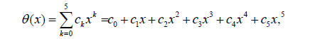 (27)
(27)
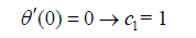
The given answer function has the constant coefficients c0 to c5 which can easily be computed by applying the initial conditions from Eq. (6). It is notable that the more numbers of series sentences of Eq. (27), the more precise the answer, and the answer is tended to the exact solution [19]. For example, solving to differential Eq. (7) by used Akbari-Ganji’s Method with (N=1, ε1=0, ε2=0.2).
In AGM, the boundary conditions are applied in two ways:
a) Applying the boundary conditions on Eq. (27) is expressed as follows:
 (28)
(28)
So the boundary conditions are applied with respect to Eq. (28) as follows:
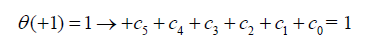 (29)
(29)
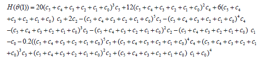
b) Boundary conditions are applied on Eq. (26), shown by H (x), and also on their derivatives as
 (30)
(30)
Eq. (30) means that the answer functions are substituted into the set of Eq. (26) instead of the dependent parameter θ, and then the boundary conditions are applied on them as follows:
 (31)
(31)
 (32)
(32)
Applying the boundary conditions on the derivatives of the set of differential equations is done in the following forms:
 (33)
(33)
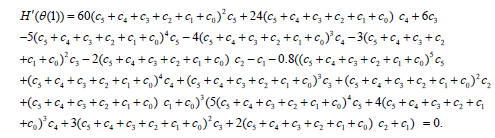 (34)
(34)
By solving a set of algebraic equations which is consisted of six equations with six unknowns from Eq. (29) and Eqs. (31)- (34), the constant coefficients of Eq. (27) can easily be gained.
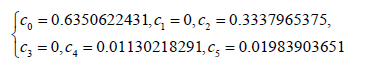 (35)
(35)
By substituting the achieved constant coefficients into Eq. (27), the solution of the set of nonlinear differential equation is gained as follows:
 (36)
(36)
Homotopy Perturbation Method (HPM)
In this section, we will apply the HPM to nonlinear ordinary differential Eq. (7). According to the HPM, we construct a homotopy suppose the solution of Eq. (7) has the form:
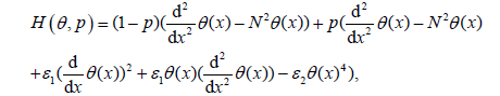 (37)
(37)
We consider θ(x) as follows:
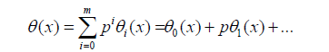 (38)
(38)
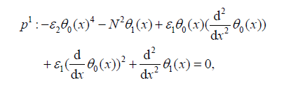
Substituting Eq. (38), into Eq. (37), and some simplification and rearranging on powers of P- terms, we have:
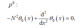 (39)
(39)
And boundary conditions are:
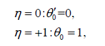 (40)
(40)
 (41)
(41)
And boundary conditions are:
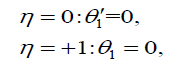 (42)
(42)
Solving Eqs. (40) and (41) with boundary conditions:
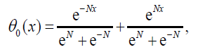 (43)
(43)
 (44)
(44)
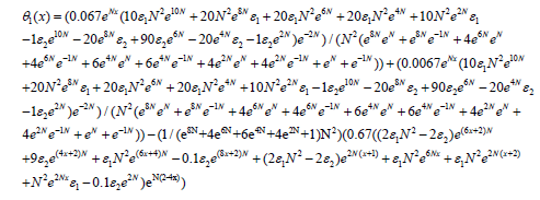
In the same manner, the rest of components were obtained by using the Maple package, that we obtain (Eq. (38)) parameters of it. According to HPM, we can conclude:
 (45)
(45)
Solution whit FlexPDE software:
In this study, we first introduce the FlexPDE software. FlexPDE software is a powerful tool for making connection among mathematical model, numerical solution and graphical results. This software has ability to analyze the wide range of engineering problems such as tension, chemical reaction kinetic and modeling of real mathematical problems. The steps of solving the problem in this software are as below:
• Initial analysis of equation.
• Formation of derivations, integrals and functions with Galerkin Finite Element method.
• Construction of coupling matrix and solving it.
• Response graphical presentation.
Also, the problems that FlexPDE is capable of solving. Problems such as first or second order partial differential equations in (one, two or three) dimensional Descartes and geometry, one-dimensional spherical or cylindrical geometry, sustainable or transition system [20], linear or non-linear equations, eigenvalues problems, and several other issues are the problems that this simple software is able to solve.In this paper, we compare the results of FlexPDE software with obtained results from HPM and AGM by writing FlexPDE software codes for Eq. (7).
Results And Discussion
Comparison of FlexPDE software results and HPM results with results of AGM
In this paper, the analytical study on Nonlinear Heat Transfer Equation in a straight fin by using Akbari-Ganji’s Method (AGM) and Homotopy Perturbation Method (HPM) to obtain an explicit solution of heat transfer equation (Figure 1). Figure 2 shows the comparison between the results of AGM method, HPM method and Flex-PDE software. In accordance with the observed figure error is very low between the results, this means there is complying between the FlexPDE software, AGM and HPM methods. Comparison between the Numerical results and AGM for different values of active parameters is shown in Table 1. In addition to, in order to verify Figure 2, comparison between the results of AGM method and HPM method is shown in Table 2. As seen in these Tables, for different values of x in the range of [0.1] error rate is very low, the slight error in Tables 1 and 2 indicates that AGM is a high accuracy method to solve these issues. Table 3 shows the Comparison between the timing of the HPM results and AGM solution for different values of active parameters. Scheduling table shows AGM solution is faster than HPM method. In addition, in this study the effect of small parameters such as a1, a2 and N, temperature distribution in convective–radiative conduction fins with variable thermal conductivity examined. Figure 3 shows the effect of parameter (a1) on temperature distribution in convective–radiative conduction fins with variable thermal conductivity. According to the Figure 3, by increasing of ε1 the value of temperature distribution increases. Also, the effects of the parameter (a2) on temperature distribution in convective-radiative conduction fins with variable thermal conductivity is shown in Figure 4. In this figure, by increasing of a2 the value of temperature distribution increases. Variation of the fin efficiency with the thermo-geometric fin parameter for different values of the thermal conductivity is shown in Figure 5. This figure shows by increasing N efficiency decline. In contrast to, with increasing of a1, a2 the value of efficiency increases. In addition, Figure 6 shows temperature distribution in convective-radiative conduction fins with variable parameter N, it is obvious that fig by increasing N temperature distribution decline.
| N=1, e1=0.2, e2=0.2 | N=2, e1=0.5, e2=0.5 | |||||
|---|---|---|---|---|---|---|
| x | Nu | AGM | Error | Nu | AGM | Error |
| 0.0 | 0.667014 | 0.666532 | 0.000482 | 0.335800 | 0.334233 | 0.001567 |
| 0.2 | 0.679514 | 0.679028 | 0.000486 | 0.358500 | 0.357403 | 0.001097 |
| 0.4 | 0.717400 | 0.716910 | 0.000490 | 0.430000 | 0.428734 | 0.001266 |
| 0.6 | 0.781855 | 0.781390 | 0.000465 | 0.553000 | 0.553496 | -0.000500 |
| 0.8 | 0.874972 | 0.874627 | 0.000345 | 0.739000 | 0.740049 | -0.001050 |
| 1 | 1.000000 | 1.000000 | 0.000000 | 1.000000 | 1.000000 | 0.000000 |
Table 1: Comparison between the numerical results and AGM solution for Θ (x).
| N=1.5, e1=0.3, e2=0.3 | N=2, e1=0.6, e2=0.7 | |||||
|---|---|---|---|---|---|---|
| x | HPM | AGM | Error | HPM | AGM | Error |
| 0.0 | 0.473480 | 0.473420 | 6.00e-05 | 0.348000 | 0.346145 | 0.001855 |
| 0.2 | 0.492404 | 0.492429 | -2.50e-05 | 0.371000 | 0.369370 | 0.001630 |
| 0.4 | 0.550154 | 0.550448 | -0.000294 | 0.441000 | 0.440571 | 0.000429 |
| 0.6 | 0.649751 | 0.650524 | -0.000773 | 0.563000 | 0.564159 | -0.001159 |
| 0.8 | 0.796622 | 0.797812 | -0.001190 | 0.745000 | 0.747202 | -0.002202 |
| 1 | 1.000000 | 1.000000 | 0.000000 | 1.000000 | 1.000000 | 0.000000 |
Table 2: Comparison between the HPM results and AGM solution for θ (x).
| Time(s) | ||
|---|---|---|
| Active Parameters | HPM | AGM |
| N=1, e1=0.2, e2=0.2 | 22.83s | 17.28s |
| N=1, e1=0.3, e2=0.3 | 27.32s | 19.76s |
| N=1, e1=0.5, e2=0.5 | 27.54s | 21.34s |
| N=2, e1=0.2, e2=0.2 | 35.36s | 28.26s |
| N=2, e1=0.5, e2=0.5 | 39.21s | 31.85s |
| N=2, e1=0.7,e2=0.7 | 41.86s | 34.94s |
Table 3: Comparison between the timing of the HPM results and AGM solution for different values of active parameters.

Figure 2: The comparison of the results obtained by AGM, HPM and Flex-PDE.

Figure 3: Temperature distribution in convective–radiative conduction fins with variable thermal conductivity for ε2=0.3, N=1.

Figure 4: Temperature distribution in convective–radiative conduction fins with variable fin dimension for ε1=0.3, N=1.

Figure 5: Variation of the fin efficiency with the thermo-geometric fin parameter for different values of the thermal conductivity parameter for the first example.

Figure 6: Temperature distribution in convective–radiative conduction fins with variable parameter N.
Conclusion
In the present study, the Akbari-Ganji’s Method (AGM) has been successfully implemented to find the solution of nonlinear heat transfer equations. The results are shown graphically. The comparison of the results of AGM with the results of the HPM, the fourth-order Runge- Kutta Numerical Method (NUM) and FlexPDE software results was conducted. This research shows that AGM is powerful method to solve nonlinear differential equations. Also, the impact of various physical parameters such as a1, a2 N are examined. Results show that a1, a2 has direct relationship with temperature distribution but N has reverse relationship with them.
References
- Kraus AD, Aziz A, Welty JR (2002) Extended Surface Heat Transfer. John Wiley & Sons.
- Aziz A, Huq SE (1975) Perturbation solution for convecting fin with variable thermal conductivity. J Heat Transfer 97: 300-301.
- Razani A, Ahmadi G (1977) On optimization of circular fins with heat generation. J Frankl Inst 303: 211–218.
- Yu LT, Chen CK (1999) Optimization of circular fins with variable thermal parameters. J Frankl Inst 336: 77-95.
- Bouaziz MN, Aziz A (2010) Simple and accurate solution for convective–radiative fin with temperature dependent thermal conductivity using double optimal linearization. Energy Convers Manag 51: 2776-2782.
- Bouaziz MN, Rechak S, Hanini S, Bal Y, Bal K (2001) Étude des transferts de chaleur non linéaires dans les ailettes longitudinales. Int J Thermal Sci 40: 843-857.
- Aziz A, Khani F (2011) Convection–radiation from a continuously moving fin of variable thermal conductivity. J Frankl Inst 348: 640-651.
- Ghasemi SE, Hatami M, Ganji DD (2014) Thermal analysis of convective fin with temperature-dependent thermal conductivity and heat generation. Case Studies in Thermal Engineering 4: 1-8.
- Joneidi AA, Ganji DD, Babaelahi M (2009) Micropolar flow in a porous channel with high mass transfer. International Communications in Heat and Mass Transfer 36: 1082-1088.
- Domairry G, Fazeli M (2009) Homotopy analysis method to determine the fin efficiency of convective straight fins with temperature-dependent thermal conductivity. Communications in Nonlinear Science and Numerical Simulation 14: 489-499.
- Domairry DG, Mohsenzadeh A, Famouri M (2009) The application of homotopy analysis method to solve nonlinear differential equation governing Jeffery–Hamel flow. Communications in Nonlinear Science and Numerical Simulation 14: 85-95.
- Ganji DD, Fazeli M (2009) Homotopy analysis method to determine Magneto the fin efficiency of convective straight fins with temperature–dependent thermal conductivity. Communications in Nonlinear Science and Numerical Simulation 14: 489-499.
- Ganji DD (2006) The application of He's homotopy perturbation method to nonlinear equations arising in heat transfer. Physics letters A 355: 337-341.
- Hatami M, Ganji DD (2014) Natural convection of sodium alginate (SA) non-Newtonian nanofluid flow between two vertical flat plates by analytical and numerical methods. Case Studies in Thermal Engineering 2: 14-22.
- Sheikholeslami M, Ganji DD (2015) Nanofluid flow and heat transfer between parallel plates considering Brownian motion using DTM. Comput Meth Appl Mech Eng 283: 651-663.
- Tari H, Ganji DD, Babazadeh H (2007) The application of He's variational iteration method to nonlinear equations arising in heat transfer. Phys Lett A 363: 213-217.
- Hashim I (2006) Adomian decomposition method for solving BVPs for fourth-order integro-differential equations. J Computational Appl Math 193: 658-664.
- Ahmadi A (2015) Nonlinear Dynamic in Engineering by Akbari-Ganji’s Method. Xlibris Corporation.
- Sheikholeslami M, Ganji DD (2014) Three dimensional heat and mass transfer in a rotating system using nanofluid. Powder Technology 253: 789-796.
- Sheikholeslami M, Hatami M, Ganji DD (2014) Nanofluid flow and heat transfer in a rotating system in the presence of a magnetic field. J Mol Liq 190: 112-120.
Citation: Akbari N, Ganji DD, Gholinia M, Gholinia S (2016) Analytical and Numerical Study to Nonlinear Heat Transfer Equation in Strait Fin. Innov Ener Res 5: 148.
Copyright: ©2016 Akbari N, et al. This is an open-access article distributed under the terms of the Creative Commons Attribution License, which permits unrestricted use, distribution, and reproduction in any medium, provided the original author and source are credited.
Select your language of interest to view the total content in your interested language
Share This Article
Recommended Journals
Open Access Journals
Article Usage
- Total views: 4600
- [From(publication date): 0-2016 - Jul 12, 2025]
- Breakdown by view type
- HTML page views: 3551
- PDF downloads: 1049