Efficiency Analysis with Different Models: The Case of Container Ports
Received: 08-Mar-2018 / Accepted Date: 20-Mar-2018 / Published Date: 24-Mar-2018 DOI: 10.4172/2155-9910.1000250
Abstract
This paper estimates and compares the technical efficiency of the container ports using data envelopment analysis (DEA) and stochastic frontier analysis (SFA) models and check the role of the characteristics of infrastructure on container port efficiency. The comparisons are based on cross-sectional data for 26 world’s major container ports in 2015 using an input variables related to the characteristics of port infrastructure, such as: the total quay length (meter), the maximum alongside depth (meter), the total terminal area (square meter) and the storage capacity thousand Twenty-foot equivalent unit (thousand TEU/year). The result represents the mean DEA-SFA efficiency differential. DEA-BCC model results indicate that 16 container ports have more than 0.5 score efficiency while with the SFA models all container ports achieved score efficiency more than 0.5. The results show that SFA models improve the score technical efficiency of the container ports. The most efficient container ports in 2015 are Shanghai and Shenzhen achieved the high value technical efficiency with an undetectable difference.
Keywords: Technical efficiency; DEA; SFA; World’s major container ports
Introduction
Container ports efficiency is an important factor to stimulate competitiveness and regional development. With the growth of the international sea traffic and the technology changes in the maritime transport industry seaports are obliged to provide progressive technology [1]. They became forced to improve port efficiency to provide comparative advantages that will attract more traffic. Thus, the global container transportation system was developed rapidly since its inauguration in the 1960, this is caused by the continued increase in the size of container ships, the automation in cargo handling systems and the continued specialization of container terminals [2].
According to [3] containerization has stimulated shipping services globalization through the emergence of alliances and acquisitions in the liner industry. In the literature of transport studies, there are two intentions to study economic performance: gross measures of productivity and shift measures of technical change [4]. The approaches of measurement efficiency include, original least squares (OLS), corrected original least squares (COLS), data envelopment analysis (DEA), and stochastic frontier analysis (SFA). Table 1 summarized the advantages and disadvantages of each method.
| Advantages | Disavantages | |
|---|---|---|
| DEA | -no a prioristructural assumption is placed on the production process | -non parametric and deterministic approach - does not consider random noise and not allow statistical hypothesis to be contrasted -does not include error term and not require specifying a functional form -sensitive to the number of variable measurements |
| SFA | -it reveals information about the production technique and distinguishes between different variables roles affecting output; -it considers statistical noise and hence it is possible to test the validity of certain assumptions and hypotheses; -it makes great flexibility in specifying the production technology (functional form); -it can model the effects of environmental/exogenous variables. |
- it need to impose an a prioristructure when constructing the frontier functional form; -the assumptions concerning the distribution of the inefficiency term have to be imposed in order to decompose the error. |
Table 1: The advantages and disadvantages of each method.
The frontier approach has different advantages and weaknesses. First, calculate an efficient frontier production is feasible in large-scale benchmarks with time series data. Second, among the main critiques of these methodologies, is the fact that measurement error has a role in the results and that stochastic frontier might deliver biased estimates due to problems with the specification under the production technology [5].
This study is established to evaluate the technical efficiency of the major container port in 2015, proving the relation between TEU(s) and variables that indicate the characteristics of infrastructure. It is expected to realize the DEA-CCR [6], DEA-BCC [1], half normal and truncated normal distribution for the SFA with cross-sectional data. The study of port efficiency has been applied in several cases of the world. A number of studies founded different results. It is obviously expected that in the case of the container port, the port should be efficient in all applications for an output orientation; because it would be desirable to maximize the number of containers. Thus, does this suggestion is valid in the case of the major container ports in the world? The background of this study is to estimate the technical efficiency of the world’s major container port. According to the estimation, we try to answer the following questions: are the characteristics of the infrastructure influencing the efficiency of the container port? Does the number of the throughput produced is the most important in the case of the container port, i.e. what is the most important the quality of the infrastructure or the number of the throughput produced in the efficiency of the container port? Another contribution of this study is to specify where the most efficient container ports are located? Then, why are these containers ports are more performing? Do the different models (DEA; SFA) produce similar efficiency rankings of container ports? Which models will be more prefer in this case?
In addition, to understand why some container ports are more efficiency than others and where the more efficient container ports are located. To answer all these questions, this paper is structured as follows: section 2 educates the survey literature concerning international container ports efficiency. Section 3, represent the methodology which examines the models, the data and the variables, and then estimate the technical efficiency with the different models concerned this study. Section 4, compare the results between container ports and prove which models are more preferable to improve efficiency levels, and then compare the founded results with the results of the literature research. Section 5, represents the conclusion and the perspective.
Literature Review
A few empirical studies that are focused on the subject of international container ports efficiency, however, there is inadequate literature that has attempted to quantitatively examine the evolution of ports efficiency with mixed results.
The most popular method used on non-parametric methodology is the DEA approach and the method most used of parametric methodology is the SFA approach. It focused that for the container ports only some studies are founded, the majority of these studies used DEA and cross-sectional data this confirms the observation that the DEA is the admired approach to measure the efficiency of the container port. This is cited also by Schoyens [7] concluded that the DEA approach is more popular than SFA. Then, it has been used more recently in applications across studies and dominates the literature. As we can see in Table 2, cross-sectional data and panel data are the types of data commonly used in the literature. However, the cross-sectional data are generally collections of multiple ports on a single point in time.
| Authors | Ports | Data Type | Year of data | Model | Mean score efficiency |
|---|---|---|---|---|---|
| [29] | 31 world ports | Cross-sectional | 1998 | DEA-CCR | 0.572 |
| [30] | 57 international container ports | Cross-sectional | 1999 | DEA-BCC | 0.763 |
| [3] | 25 of 30 largest container ports in the world | Panel | 1992-1999 | CCR – Window | 0.722 |
| [31] | 25 of the 30 largest container ports plus 5 mainland China | Cross-sectional | 1992 | DEA-CCR | 0.689 |
| [23] | 27 international container ports | Panel | 1999-2002 | DEA-CCR DEA-BCC SFA production frontier |
0.735 |
| [25] | 25 container ports/terminals, | Cross-sectional | 1999 | Cobb-Douglas production function |
0.866 |
| [26] | 57container ports which 30 ranked in the top | Cross- sectional | 2001 | DEA-CCR DEA-BCC SFA production frontier |
0.580 |
| [26] | 74 European container port |
Cross- sectional |
2002 | SFA Cobb-Douglas production function | 0.723 |
| [32] | 10 Container ports in Asia-Pacific region | Cross-sectional | 1998 | DEA-CCR | 0.830 |
| [33] | 77 world container ports | Cross-sectional | 2007 | DEA-BCC | 0.667 |
| [10] | 25 leading container ports | Panel | 1992-1999 | BCC- Window | 0.785 |
| [9] | 20 largest Container ports in 20 countries | cross-sectional | 2005 | DEA-CCR DEA-BCC |
0.740 |
| [34] | 77 global container ports | Cross-sectional | 2003 | DEA-CCR | 0.563 |
| [11] | 69 major Asian containers ports | Cross-sectional | 2007 | DEA | 0.484 |
| [12] | 16 container terminals in Turkey and counterparts region | Panel | 2006-2008 | DEA-CCR DEA-BCC |
0.565 0.788 |
| [13] | 30 Europe container ports | Cross sectional | 2008 | DEA-CCR DEA-BCC |
0.417 0.658 |
| [35] | 21 China and Asian container ports | Panel data | 2003-2007 | DEA-CCR | 0.793 |
| [7] | 6 Norwegian and 18 other Nordic and UK ports | Panel data | 2002-2008 | DEA-CCR DEA-BCC |
0.820 |
| [14] | 33 Asian Pacific Region |
Panel data | 2003-2010 | DEA-CCR DEA-BCC |
0.274 0.596 |
| [15] | Chinese container terminals | Panel data | 2006-2011 | DEA-Malmquist | - |
| [16] | 21 SMP terminals in china | panel | 2008-2012 | DEA-CCR DEA-BCC |
0.430 0.848 |
| [17] | 19 container terminals in the Middle Eastern region. | Cross sectional | 2012 | DEA-CCR | 0.634 |
| [27] | 21Asien container ports | Cross sectional | 2011 | DEA | 0.734 |
| [18] | Container port in china and 5 west Africa | panel | 2008-2013 | DEA | - |
Table 2: Studies Efficiency in international container ports sector [3,7,9-18,23,25-27,29-35].
Most of the previous studies accept container throughput (TEUs) as the output variable of efficiency measurement. The most inputs used are physical variables. Even so, the variations in crane and handling technology are hardly captured in the literature [8].
The study of the top container ports is related to the international geographical location. The sample with international ports is more significant. However, the samples are usually chosen among the top container ports by throughput (TEUs). The focusing on these kinds of samples, founded that is composed of the huge container ports. These views are expressed by several studies such as Wu and Goh [9], Cullinane and Wang [10].
There are different manners to use the parametric and nonparametric methods for measurement efficiency in the ports sector. Thus, this paper remains only the studies which educated the efficiency of the container ports to keep the capability of comparing the results. Therefore, describes the real status and the characteristics of the picked container ports.
The different studies about container ports efficiency use the same output (TEUs), however the input variables are different. The majority of study selected the infrastructure or the superstructures factors as input variables of the ports. Studies in Table 2 reveal that, to the extent of 2010, the majority of search about container ports was developed by Cullinane in several years. Furthermore, the examination of these studies, of cullinane appeared that they used the same variables only changing the type of data, the sample or the models. After 2010, many researches are developed as Table 2 describe. The analysis of these researches proves that the majority of studies are regional not international for example the studies [11-19] takes the case of Asian container ports and specially china ports which prove that the interesting container port are located in the Asian country and china ports occupied the first rank after 2010. A number of studies in container ports educate the European container ports case as the studies [7,8,13].
The analysis of researchers showed also a various result. For instance, the studies [11,13,17] used DEA models with cross-sectional data, they found a small average efficiency less than 0.5 in some cases. Furthermore, the studies [7,16,18] used panel data and found an average efficiency more than 0.8, which demonstrate the important effect of the type data for improving efficiency measurement.
Methodologies
The productivity and technical efficiency concepts are illustrated in Figure 1 [20] which describes a simple production process involving a single output (y) and a single input (x). Points A, B and C define the relationship between input and output of three different firms and these points represent the productivity level of each firm respectively. Firms that produce outputs on the production frontier are operating at maximum possible productivity and are recognized as technically efficient.

Figure 1: Production frontier and technical efficiency Source: Coelli et al, 1998.
Firms produce under the frontier line are considered to be technically inefficient [5]. Thus, firms which operate at points B and C on the production frontier are considered technically efficient firms. The firm operated at point A is considered inefficient because it could increase its productivity by moving from output Y1 to maximum productivity at output Y2. The firm at point C produces output level Y1 by using a lower input level X1, while firm produces the same output level Y1 by using more inputs. Accordingly, firm A is considered as a technically inefficient firm. Technical efficiency is recognized by operating at maximum possible production, given the input level. The production frontier shows all points of technical efficiency [5].
Similarly [5] illustrated the difference between output and input orientation measurement. This paper used output orientation for the production function frontier. The Figure 2 represents the output oriented efficiency.

Figure 2: Output oriented efficiency measures Source: Coelli et al, 1998.
According to the Figure 2, the production frontier is represented by the isoquant ZZ’. The technical inefficiency of the firm defined by the point A can be measured by the distance AB. It corresponds to the output proportions that can be increased without changing the input level. The measurement of the technical efficiency oriented output is defined by the ratio ET=OA/OB
Data envelopment analysis (DEA)
The method DEA is a non-parametric technique to estimate a production frontier based on the output and input observations for a group of DMUs (Decision-Making Units) [21]. The resulting frontier comprises efficiently operating DMUs and is said to envelop the other DMUs that rest below the frontier and in relative terms are operating inefficiently.
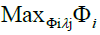
In the present context, container ports serve as decision-making units. Each container port is producing an output, y, using a K inputs. Using standard notation, the formal output-oriented DEA model for thecontainer port can be stated as follows:
 (1)
(1)
 (2)
(2)
 (3)
(3)
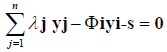
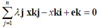
Where j=1, n is the container ports, the s and e are output and input slacks (both being ≥ 0), and ϕi measures the increase in output potential for each container port. Hence, ϕi ≥ 1.The weights,λ, on outputs and inputs give rise to variable returns to scale (VRS) in production and are due to Banker [1]. In this case, the underlying technology of production can be one of increasing, decreasing, or constant returns to scale. The more restrictive constant returns to scale (CRS) model originally developed by Charnes [6] eliminates the last equation (3). The technical efficiency with which each container port is based on its actual production accomplishment relative to its estimated production level for the frontier.
 (4)
(4)
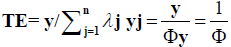
Technical efficiency, therefore, varies in the range 0 ≤ TE ≤ 1 with the value of one representing efficient container ports on the frontier. Technical efficiencies estimated under the (CRS) model will be less than or equal to the technical efficiencies coming from the more flexible (VRS) model. It is customary to estimate both efficiencies and use the results to compute scale efficiency (SE) as the ratio of CRS to VRS efficiencies. That practice will be followed in the empirical analysis of this paper. If SE=1, then a container port is operating at the most efficient scale. A SE less than one would be due to decreasing returns to scale (over production) or increasing returns to scale (under production).
Stochastic frontier models specification
The measurement of container port technical efficiency is based upon deviations of observed from the efficient production frontier. The technical efficiency estimation using stochastic frontiers is an outputorientated measure, which takes a value between 0 and 1.
A stochastic frontier model is considered as follows by Battese and Coelli [22] with a simple specification of time-unvarying port effects which incorporates for the cross-sectional data associated with observations of a sample of N ports.
The different distribution assumptions on the inefficiency term U result in two cross-sectional models: Half Normal and Truncated Normal distribution. The models are defined as follows:
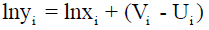 (5)
(5)
| Where: | |
| yi | is the output obtained by the i-th port; |
| xi | is the vector of input quantities of the i-th port; |
| Β | is the vector of parameters; |
| Vit | are random variables representing statistic noise, which are assumed to be independent and identically-distributed (i.i.d.) N(0, σv2), |
| Uit | are non-negative random variables representing technical inefficiency, which can be assumed i.i.d. either 1) |N(0, σu2)| - Half Normal distribution; or 2)truncations at zero of the N (µi, σu2)–Truncated Normal distribution |
| σv | is the variance parameter of noise term; |
| σu | is the variance parameter of inefficiency term; |
| Σ | is the combined error term; |

If γ is close to zero, it indicates that the deviations from the frontier are due mostly to noise. If γ is close to one, it indicates that the deviations from the frontier are due mostly to the technical inefficiency.
The ML estimators of β2 and γ will be determined by the calculation of the maximum of the likelihood function presented by Battese and Coelli [1]. The software Frontier 4.1obtains the estimates of the former parameters through three steps and gives estimate of the technical efficiency of each container port. The Likelihood Ratio (LR) test is:
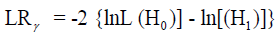 (6)
(6)
Where L (H0) is the value of the likelihood function under H0 and L (H1) is the value of the likelihood function under H1.
The LRγ statistic has asymptotic distribution, which is a mixture of the chi-square distributions, whose critical values were taken from Kodde and Palm [19]. If LRγ>χ2m, H0 will be refused for a test of size α. The “m” index refers to degrees of freedom corresponding to the number of restrictions. If the null hypothesis is not rejected then the term of inefficiency should be removed from the model and the model can be estimated by the OLS method. As 0≤γ≤1, so γ=1 is the same as σV2=0, therefore the stochastic frontier model is not different from the deterministic frontier model, that is, there are no random errors in the production function, all deviations are due to inefficiency.
The density function of U in the case of the half normal distribution is:
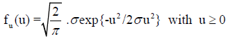 (7)
(7)
The density function of U in the case of the truncated normal distribution is:
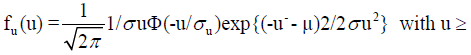 (8)
(8)
Where, Φ (.) stands for the standard normal distribution function.
The logarithmic stochastic frontier model specified for the container ports sector in the cross-sectional case is conducted by assuming the appropriateness of the log-linear Cobb–Douglas function. The use of the specification of the SFA models are in logs to assume a liner functional form, accordingly, to estimate the Cob-Douglas production function, it need to log the inputs and outputs data.
Variables and data description
The main objective of the container port is to maximize the traffic of containerization. Therefore, the container, as new technology, can improve port efficiency. Consequently, the output variable selected for this study is the number of containers in TEUs. The selected input variables are related to the characteristics of port infrastructure, such as: the total quay length (meter), the maximum alongside depth (meter), the total terminal area (square meter) and the storage capacity (thousand TEU/ year). These variables are selected according to the available data for the various container ports. The sample comprises the major 26 container ports in 2015 according to the containers traffics measured in TEUs. The data of the throughput are collected from the Lloyd’s Ports of the World (report of 2016), for the other variables the data are collected according to several source such as: the annual statistics report of container port (2015), Port of Hong Kong in 2015, the annual statistical of the China Ports Association (2015) and the various official websites of container ports. The Figure 3 and Table 3 describe the container number produced by (TEUs, 000) in 2015 with the real rank of each port. The first container port is Shanghai, it is container number is more than 36000 (TEUs, 000) and the less one is Tanjung Periok with a container number more than 5000.

Figure 3: Container ports and their number of production by (TEUs, 000) in 2015.
| Ports | Country | Region | (TEUs, 000/2015) | |
|---|---|---|---|---|
| 1 | Shanghai | China | Asia | 36537 |
| 2 | Singapore | Singapore | Asia | 30922 |
| 3 | Shenzhen | China | Asia | 24204 |
| 4 | Ningbo | China | Asia | 20620 |
| 5 | Hong kong | China | Asia | 20114 |
| 6 | Busan | South Korea | Asia | 19469 |
| 7 | Guangzhou | China | Asia | 17625 |
| 8 | Qingdao | China | Asia | 17510 |
| 9 | Dubai | UAE | Middle East | 15592 |
| 10 | Tianjin | China | Asia | 14100 |
| 11 | Rotterdam | Netherlands | Northern Europe | 12235 |
| 12 | Port klang | Malaysia | Asia | 11890 |
| 13 | Kaohsiung | Taiwan | Asia | 10264 |
| 14 | Antwerp | Belgium | Northern Europe | 9654 |
| 15 | Dalian | China | Asia | 9450 |
| 16 | Xiamen | China | Asia | 9183 |
| 17 | Tanjungpelepas | Malaysia | Asia | 9120 |
| 18 | Hamburg | Germany | Northern Europe | 8821 |
| 19 | Los angeles | US | NorthAmerica | 8160 |
| 20 | Long beach | US | NorthAmerica | 7192 |
| 21 | Leamchabang | Thailand | Asia | 6780 |
| 22 | New york | US | NorthAmerica | 6372 |
| 23 | Yingkou | China | Asia | 5922 |
| 24 | Ho chi minh | Vietnam | Asia | 5788 |
| 25 | Bremen | Germany | Northern Europe | 5300 |
| 26 | Tanjungperiok | Indonesia | Asia | 5201 |
Table 3: Container ports with their throughput (TEU, 000s) handled in 2015.
According to the Figures 4 and 5 and the distribution of throughput (TEUs, 000) containers varies between countries and regions. The region of Asia, especially the China countries, handled the most number on containers in 2015. It is always reminded that this analysis is only for the 26 major ports. The 26 ports cannot be representative of the whole world, it can present only a part.

Figure 4: Division of the throughput (TEUs, 000) in 2015 between the countries.

Figure 5: Division of the throughput (TEUs, 000) in 2015 between the regions.
Table 4 shows the descriptive statistics for different variables. The minimum value and the maximum value of throughput (TEU, 000s) are 36537 and 5201, respectively, with a standard deviation of 8097, 46886, indicating that regional development is very unbalanced. The variable total quay length, the maximum and minimum are 14120 and 3590. The maximum alongside depth varies from 16 to 19, with a standard deviation of 0.646. The total terminal area is large. The minimum value and the maximum value of the total terminal area are 10570 and 2000, respectively, with a standard deviation of 2279,543. The storage capacity ranges from 15 to 555 thousand TEU, 000s /year, with a standard deviation of 0.13.
| Y | X1 | X2 | X3 | X4 | |
|---|---|---|---|---|---|
| Mean | 13385.576 | 9185.807 | 17.538 | 5410.115 | 310.923 |
| Maximum | 36537 | 14120 | 19 | 10570 | 555 |
| Minimum | 5201 | 3590 | 16 | 2000 | 15 |
| Std. Dev. | 8097.469 | 2855.649 | 0.649 | 2279.543 | 105.309 |
| Observations | 26 | 26 | 26 | 26 | 26 |
Table 4: Descriptive analysis data.
Results
The results achieved according to the Ordinary Least Square (OLS) and the maximum likelihood (MLE) estimates of the parameters production function were obtained from the software frontier 4.1. Table 5 shows that the maximum-likelihood estimate of the parameter of the total quay length input are -0.278 and -0.282 for the half vs. truncated normal distributions respectively. For both distributions the coefficient of the total quay length was found to be insignificant. The coefficients of the variables maximum alongside depth, total terminal area and the total container storage capacity are observed as significant in the two cases of distribution. Hence, there is a direct effect observed in the container ports production.
| Variables/parametres | OLS | MLE | |
|---|---|---|---|
| half normal | Truncated normal | ||
| Constant | -0.212 (-0.265) | -0.179 (-0.283) | -0.208 (-0.636) |
| X1 | -0.280 (-0.121) | -0.278 (-0.123) | -0.282 (-0.435) |
| X2 | 0.158 (0.674) | 0.156 (0.895) | 0.157 (0.606) |
| X3 | 0.566 (0.168) | 0.563 (0.184) | 0.567 (0.634) |
| X4 | 0.167 (0.425) | 0.165 (0.487) | 0.166 (0.392) |
| sigma-squared (σ2) | 0.236 | 0.192 | 0.194 |
| Gamma (γ) | 0.406 | 0.500 | |
| Mu | 0 | -0.321 | |
| Eta | 0 | 0 | |
| log likelihood | 0.166 | 0.165 | |
Table 5: The OLS and the MLE of the Stochastic Frontier Function.
For both the half-normal and the truncated-normal distribution, γ=σU2/(σV2+σU2)is estimated at 0.406and 0.50 levels, respectively, that is mean 40.6 percent of random variations in the half normal distribution in container port production are due to the inefficiency. Also, 50 percent of random variations in the truncated normal distribution in container ports production are owed to the inefficiency. It is evident that the estimates of σ2 amount of 0.192 and 0.194 for half vs. truncated normal distributions respectively. They are observed significant in the both cases of half vs. truncated normal distributions.
The estimate of the η (named (Mu) in the Table 3) parameter is found negative (i.e. η=-0.321). The parameter η is negative, indicating that the distribution of the inefficiency effects is concentrated around zero, as compared with half-normal distribution.
The values of the log likelihood function for the two distribution production functions are 0.166 and 0.165, respectively as Table 5 present. There is a little difference between the two results not exceed 0.001.
The average efficiencies and other descriptive statistics of the efficiency distributions are shown in Table 6 and Table 7 shows the efficiency estimates obtained from the DEA models and makes comparisons to those that are derived from the SFA estimates.
| DEA | SFA | ||||
|---|---|---|---|---|---|
| DEA-CCR | DEA-BCC | Scale | Half normal | Truncated normal | |
| Mean | 0.325 | 0.616 | 0.565 | 0.871 | 0.876 |
| Median | 0.248 | 0.595 | 0.501 | 0.876 | 0.886 |
| Maximum | 1.000 | 1.000 | 1.000 | 0.998 | 0.999 |
| Minimum | 0.064 | 0.079 | 0.219 | 0.718 | 0.722 |
| Std. Dev. | 0.245 | 0.340 | 0.239 | 0.088 | 0.087 |
Table 6: Descriptive statistics of efficiency estimates.
| DEA | SFA | ||||||
|---|---|---|---|---|---|---|---|
| Ports | CCR | BCC | scale | Returns to scale | Half normal | Truncated normal | |
| 1 | Shanghai | 1.000 | 1.000 | 1.000 | - | 0.998 | 0.999 |
| 2 | Singapore | 0.461 | 1.000 | 0.461 | Inc | 0.995 | 0.996 |
| 3 | Shenzhen | 1.000 | 1.000 | 1.000 | - | 0.998 | 0.999 |
| 4 | Ningbo | 0.227 | 0.233 | 0.976 | Inc | 0.980 | 0.984 |
| 5 | Hong kong | 0.219 | 1.000 | 0.219 | Inc | 0.886 | 0.889 |
| 6 | Busan | 0.132 | 0.247 | 0.534 | Inc | 0.870 | 0.873 |
| 7 | Guangzhou | 0.128 | 0.189 | 0.677 | Inc | 0.920 | 0.924 |
| 8 | Qingdao | 0.125 | 0.159 | 0.782 | Inc | 0.955 | 0.957 |
| 9 | Dubai | 0.084 | 0.196 | 0.430 | Inc | 0.883 | 0.885 |
| 10 | Tianjin | 0.142 | 0.540 | 0.263 | Inc | 0.803 | 0.806 |
| 11 | Rotterdam | 0.397 | 1.000 | 0.397 | Inc | 0.882 | 0.887 |
| 12 | Port klang | 0.234 | 1.000 | 0.234 | Inc | 0.778 | 0.783 |
| 13 | Kaohsiung | 0.276 | 0.632 | 0.436 | Inc | 0.761 | 0.762 |
| 14 | Antwerp | 0.200 | 0.268 | 0.745 | Inc | 0.975 | 0.978 |
| 15 | Dalian | 0.395 | 0.483 | 0.818 | Inc | 0.990 | 0.991 |
| 16 | Xiamen | 0.524 | 0.701 | 0.748 | Inc | 0.894 | 0.897 |
| 17 | Tanjungpelepas | 0.064 | 0.079 | 0.807 | Inc | 0.897 | 0.900 |
| 18 | Hamburg | 0.416 | 1.000 | 0.416 | Inc | 0.856 | 0.864 |
| 19 | Los angeles | 0.142 | 0.363 | 0.392 | Inc | 0.763 | 0.769 |
| 20 | Long beach | 0.395 | 0.558 | 0.707 | Inc | 0.851 | 0.857 |
| 21 | Leamchabang | 0.217 | 0.735 | 0.295 | Inc | 0.866 | 0.887 |
| 22 | New york | 0.126 | 0.242 | 0.521 | Inc | 0.854 | 0.863 |
| 23 | Yingkou | 0.263 | 0.546 | 0.481 | Inc | 0.759 | 0.767 |
| 24 | Ho chi minh | 0.636 | 1.000 | 0.636 | Inc | 0.763 | 0.765 |
| 25 | Bremen | 0.324 | 0.838 | 0.387 | Inc | 0.756 | 0.758 |
| 26 | Tanjungperiok | 0.331 | 1.000 | 0.331 | Inc | 0.718 | 0.722 |
| Mean | 0.325 | 0.616 | 0.565 | 0.871 | 0.876 | ||
Table 7: Efficiency estimates obtained from the DEA and the SFA.
DEA estimation indicates that the container ports efficiencies range from 0.325 to 0.616 depending upon the constant or variable returns to scale specification. This suggests that with given more resources, container ports can, on average, increase container production by approximately 67.5% to 39%. The constant returns to scale efficiencies are lower than variable returns to scale due to the presence of scale efficiencies. Thus, the scale efficiencies are presented separately. The scale efficiency determined by the ratio of CRS to VRS efficiencies.
Generally, the DEA mean results indicate that container ports are operating considerably below their optimal capacity. The SFA efficiency estimates confirm that both the half-normal and truncated normal SFA efficiencies are more than the DEA-BCC efficiency estimate. However, for the two technical efficiency estimates, there are some highly efficient container ports. The DEA variable returns to scale efficiency is inferior to either SFA efficiency estimate. The difference is statistically significant.
The largest value DEA vs. SFA of mean efficiency is 0.616 and 0.876 respectively, which found a difference around to 0.26. In the same previous studies [23] found a value approximate to 0.766 for the DEA and 0.934 for the SFA in 2002 for 27 international container ports. Cullinane [24] found a value of mean efficiency rough to 0.783 for the DEA and to 0.790 for the SFA for 57 top container ports which 30 ranked the top in 2001. In addition, the height value is 0.866 founded by Tongzonand Heng [25] according to a Cobb-Douglas production function. The depth value efficiency is 0.484 estimated by Munisamy and Singh [11] with DEA model. The results of the studies of [14] founded a great difference between the DEA-BCC and DEA-CCR models more than 0.3.
Thus, differences in results might be attributed to the heterogeneity of the ports for the same sample. It is expected that there exists greater homogeneity among the 26 container ports relative to this case. It is also important to note that the best value of estimate efficiency it accorded to the truncated normal model distribution, which shows that the truncated distribution of the term error is able to improve container ports efficiency. Correspondingly, Almawsheki and Muhammad [17] concluded that among the 19 container terminals studies only 3 terminals such as Jebel Ali, Salalah and Beirut are efficient, the others terminals are inefficient. Besides [13] studied 30 seaports in South- Eastern Europe they founded a value around to 0.66 with the DEABCC and to 0.61 with scale efficiency scores.
The container ports efficiency results confirm that the mean efficiency is improved according to the specification models. These estimated improvements are present in all DEA and SFA models. Comparing across models, the truncated normal-SFA and DEA-BCC achieved the highest value efficiency. The differences between the SFA models can be attributed to the different distribution assumptions related to the inefficiency term, while the differences between the DEA models are due to the scale efficiencies contained in the (CRS) vs. (VRS). These scale efficiencies (SE) as reported in Table 6 remain below the value of one, therefore, indicate that container ports are on average scale inefficient.
In a separate DEA analysis, however, it was found that the container ports operate under increasing returns to scale. The increasing returns to scale apparent in both SFA estimates lend support to those findings. Yet, the DEA scale inefficiencies indicate that most container ports are producing below optimal total terminal area.
The results for the average efficiencies reflect the annual efficiency differences with the more flexible DEA-BCC model showing the larger value around to 0.616 under the DEA estimation and the truncated model showing the great value around to 0.876 below the SFA estimation.
Shanghai is the largest container port in the worldwide, handling around 36.537 million TEUs in 2015. It was the most efficient container ports in this research accompanied with Singapore, Shenzhen, Ningbo and Dalian. These five container ports achieved scale efficiency more than 0.8 with DEA models and height value with the SFA models more than 0.9. Moreover, as it is seen these best four ports are china container ports.
To compare the results with similar application in the literature, it found that the study of Cullinane and Wang [10] reveal that the two container ports of Keelung and Colombo were found to be highly efficient during the whole study period (1992-1999). This contrasts with the results for world container ports such as Rotterdam, Hamburg and Antwerp that have a large container throughput and face strong competition from other ports. The results of Munisamy and Singh [11] reveal that the Chinese container ports as Xiamen, Yantian, Lianyungang, Tianjin and Guangzhou are the most efficient. The same authors conclude that China follows the global trend in engaged liner services at ports.
The classification was based on an analysis conducted by Wang and Cullinane [26]. Ports that are classed as the most competitive comprised Rotterdam, Hamburg, Antwerp, Bremen/Bremerhaven, Los Angeles and Long Beach. During the period under the same study, the infrastructure and equipment have remained relatively stable in the ports that face little or no competition, such as in Keelung and Colombo. However, the ports of Rotterdam, Hamburg and Antwerp have invested actively in port facilities and infrastructure in order to increase the capacity and improve the productivity of their container handling capability.
The analysis of the study of Lie and Lih [22] shows that among the 27 ports, operating efficiency scores of Hong Kong is the highest and demonstrates the best performance in each model. The remaining ports show the variation of performance with different models. DEACCR has 3 efficient ports, including Hong Kong, Shenzhen, and Los Angeles, and DEA-BCC has 9 efficient ports on year 2002. In addition, for the SFA-CD (cobb-Douglas) Hong Kong, Singapore, and Busan are the most efficient, and for the SFA-TR (translog) Hong Kong, Tanjunk Priok, and Busan in top 3 efficient ports on year 2002. The Port of Tanjung Pelepas has an inferior rating in both SFA-CD (cobb-Douglas) and SFA-TR (translog) models. Infante and Gutiérrez [14] displayed that the ports of Hong Kong, Xiamen and Kaohsiung are found to be efficient independent of the returns to scale assumption. Hyun [27] found that the ports of Shanghai, Hong Kong and Qingdao revealed to be the most efficient from 21 Asian container ports acceding to the data of 2011.
The relation between the estimated efficiencies of the container ports and the number of throughput evaluation of each container port findings showed that a port efficiency level has great relations with the quantities of container production. The representation in Figures 6 and 7 of the scale efficiency and the score efficiency of truncated normal distribution, which present the height value efficiency, to schematize the difference between the results detected under the two methods. It describes that the ports with larger throughput cannot achieve the best score efficiency in all the case, such as the Figures 6 and 7 shown. In addition, the Figures 4 and 5 showed the great difference between the results of scale efficiency and the truncated normal.

Figure 6: Relationship between scales efficiency value and container ports.

Figure 7: Relationship between Truncated normal score efficiency and container ports.
In this paper only 4 ports are efficient with DEA-CCR, such as Shanghai, Shenzhen, Xiamen and ho chi minh, for the DEA-BCC, 16 containers ports are efficient. Furthermore, all the container ports improved her efficiency with the SFA models. It clears that container ports are more efficient in 2015, this study found the best mean efficiency (0.876) still 2015, which prove that the container ports improve their infrastructure. The competitiveness of these ports is highly relevant for increasing the investments in infrastructure characteristics, which makes them dependent on the quality and efficiency of their hinterland connections. The Stochastic models show that the sample of container ports selected has relatively access to transport infrastructure, which makes it’s the competitive container ports in the world. The prioritization of expanding the existing infrastructure and starting new construction projects leading to an efficient container port. Subsequently, the comparisons of this research with the last researches demonstrate the difference in results.
Conclusion
This paper studied the technical efficiency of the major container ports using the DEA and SFA models. Moreover, examined the comparability between container ports ranking efficiencies and it compares also with the results of literature studies. The empirical results are very satisfactory and lead to the following conclusions:
• The models are estimated with the error components model specification. As well, the results indicated that the input variables included in the technical efficiency effects have a significant influence on container ports production, especially the variable terminal area.
• The half normal distribution is found to be similar to the truncated normal distribution for the technical inefficiency effect and the technical efficiency. Moreover, technical inefficiency effects are also positively influenced by seed within the production process.
• The average levels of technical efficiency differ considerably across the different container ports. However, both the DEA and SFA methods have signification mean efficiency, and provide an appropriate technique of treating the measurement of container ports efficiency.
• The total average of efficiency scores of SFA model with truncated normal distribution is the highest which, equal to 0.876. Thus, with the DEA-BCC and DAE-CCR models achieved a mean efficiency is equal to 0.616, 0.325, respectively. It is found that the total average scores SFA method is better than the DEA method in measuring container ports efficiency.
• The comparison between the two stochastic models that differ according to their term error distribution (half normal or truncated normal distribution). In the light of the obtained results, and following the comparison between both models, we found that the models of SFA are most relevant.
• The final part is devoted to a comparison between the deterministic method presented by the DEA model and the stochastic model. This comparison made us suppose that the SFA has the advantage of dealing with stochastic noise, allowing for statistical tests of hypotheses concerning the production structure and degree of inefficiency. Further, DEA does not impose any assumptions about production functional form and also does not take into account random errors; hence, the efficiency estimates may be biased if the production process is largely characterized by stochastic elements.
• The combination of both DEA and SFA support management to understand the efficiency of international container ports and to identify the causes of inefficiency. Furthermore, both two methods are frontier function to measure efficiencies of all firms with crosssection data, and many container ports may have characteristics of consistency for DEA and SFA. Therefore, this paper adopts both DEA and SFA methods to evaluate container ports efficiency.
• The comparison founded that the port of Shanghai, Singapore, Shenzhen, Ningbo and Dalian are the most efficient container ports, according to the four models used for evaluation, which explain the best infrastructure of these container ports with a great number of containers.
Additionally, the findings have some important implications for the sample of container ports selected. For example, the attentive analysis showed that Chinese port and Asian in general occupied the first ranked in 2015 and others was the first before 2010 now are at the end of the ranking. In addition, to the investment in infrastructure, [15] reveal that Chinese container terminals could improve technical efficiency by more effectively optimizing their corporate governance, utilizing capital available and allocating both human and natural resources. As well, this changing and development is due to the instability in the port industry as Notteboomand Winkelmans, [28] described the fierce competition and the fear for under-utilization of terminal facilities put a strong downward pressure on the levels of port dues and container handling rates.
The synthesis of our study shows that some container ports are inefficient for the applied approach DEA. Though, all the container ports are efficient for the different models. This can be explained by the importance of the term error in container port production. Which prove that seaport sector is an area where the perception errors are highly developed.
The first weakness of this study is the cross sectional data which make a difficult to determine temporal relationship between exposure and results. The second weakness appears in the number of samples, it represents only 26 ports among the 100 major ports of the world.
There are different aspects that may be considered in future extensions of the current analysis, but the most important is to classify this container port according to their criteria. Further the differentiation of terminals into transhipment, gateway and hybrid is a necessary step in port efficiency evaluation, as ports form part of different strategies and serve varied functions within the regional port system.
Acknowledgements
The author is grateful to the editor and the anonymous reviewers for their valuable suggestions and comments.
References
- Banker RD, Charnes A, Cooper WW (1984) Some models for estimating technical and scale inefficiencies in data envelopment analysis. Management Science 30: 1078-1092.
- Li KX, Luo M, Yang J (2012) Container Port Systems in China and the USA: A Comparative Study. Maritime Policy & Management 39: 461- 478.
- Cullinane K, Song DW, Ji P, Wang TF (2004) An application of DEA windows analysis to container port production efficiency. Review of Network Economics 3: 7.
- Oum TH, Tretheway MW, Waters WG (1992) Concepts, Methods and Purposes of Productivity Measurement in Transportation. Transportation Research Part A 26: 493-505.
- Mortimer D (2002) Competing methods for efficiency measurement: a systematic Review of Direct DEA vs SFA/DFA Comparisons. Centre for Health Program Evaluation (CHPE) Working Paper 136.
- Charnes A, Cooper WW, Rhodes E (1978) Measuring the efficiency of decision-making units. European Journal of Operational Research 2: 425-444.
- Schoyens H, Odeck J (2013) The technical efficiency of Norwegian container ports: A comparison to some Nordic and UK container ports using Data Envelopment Analysis (DEA). Maritime Economics & Logistics 15: 197-221.
- Bichou K (2012) An empirical study of the impacts of operating and market conditions on container-port efficiency and benchmarking. Research in Transportation Economics.
- Wu YC, Goh M (2010) Container port efficiency in emerging and more advanced markets. Transportation Research Part E: Logistics and Transportation Review 46: 1030-1042.
- Cullinane K, Wang T (2010) The efficiency analysis of container port production using DEA panel data approaches. OR spectrum 32: 717-738.
- Munisamy S, Singh G (2011) Benchmarking the efficiency of Asian container ports. African journal of business management 5: 1397-1407.
- Demirel B, Cullinane K, Haralambides H (2012) Container Terminal Efficiency and Private Sector Participation. The Blackwell Companion to Maritime Economics 571-598.
- Niavis S, Tsekeris T (2012) Ranking and causes of inefficiency of container seaports in South-Eastern Europe. European Transport Research Review 4: 235-244.
- Infante Z, Gutierrez A (2013) Port Efficiency in apec1.México y la Cuenca del PacÃfico.
- Song BB, Cui YY (2014) Productivity changes in Chinese Container Terminals 2006-2011. Transport Policy 35: 377-384.
- Ding ZY, Wang Y, Yeo GT (2015) The Relative Efficiency of Container Terminals in Small and Medium-Sized Ports in China. The Asian Journal of Shipping and Logistics 31: 231-251.
- Almawsheki E, Muhamed Z (2015) Technical Efficiency Analysis of Container Terminals in the Middle Eastern Region. The Asian Journal of Shipping and Logistics 31: 477-486.
- Tetteh EA, Yang HL, Gomina Mama F (2016) Container ports throughput analysis: A comparative evaluation of China and five West African countries. International Journal of Engineering Research in Africa 22: 162-173.
- Kodde DA, Palm FC (1986) Wald Criteria for jointly Testing Equality and Inequality Restrictions. Econometrica 54: 1243-1248.
- Coelli T, Rao DSP, Battese GE (1998) An introduction to efficiency and productivity analysis. Kluwer Academic, Boston.
- Cook WD, Zhu J (2008) Data Envelopment Analysis: Modelling operational processes and measuring productivity. Boston: Kluwer Academic Publishers.
- Battese GE, Coelli TJ (1992) Frontier Production Function, Technical Efficiency and Panel Data: With Application to Paddy Farmers in India. Journal of Productivity Analysis 3: 153-169.
- Lie-Chien L, Lih-An T (2005) Application of DEA and SFA on the Measurement of Operating Efficiencies for 27 International Container Ports, Proceedings of the Eastern Asia Society for Transportation Studies 5: 592-607.
- Cullinane KPB, Song DW (2006) Estimating the Relative Efficiency of European Container Ports: A Stochastic Frontier Analysis. Research in Transportation Economics 16: 85-115.
- Tongzon, J, Heng W (2005) Port privatization, efficiency and competitiveness: Some empirical evidence from container ports (terminals). Transportation Research Part A: Policy and Practice, 39: 405-424.
- Cullinane K, Wang TF, Song DW, Ji P (2006) The Technical Efficiency of Container Ports: Comparing Data Envelopment Analysis and Stochastic Frontier Analysis. Transportation Research 40: 354-374.
- Hyun Mi J, Ho P, Sang YK (2016) Efficiency Analysis of Major Container Ports in Asia: Using DEA and Shannon’s Entropy. International Journal of Supply Chain Management 5.
- Nottboom TE, Winkelmans W (2001) Structural changes in logistics: How will port authorities face the challenge?. Maritime Policy & Management 28: 71-89.
- Valentine VF, Gray R (2001) The measurement of port efficiency using data envelopment analysis. In: Proceedings of the 9th World Conference on Transport Research, Seoul, South Korea.
- Wang TF, Cullinane K, Song DW (2003) Container port production efficiency: A comparative study of DEA and FDH approach. Journal of the Eastern Asia Society for Transportation Studies 5: 698-713.
- Cullinane K, Ji P, Wang TF (2005a) The relationship between privatization an DEA estimates of efficiency in the container port industry. Journal of Economics and Business 57: 433-462.
- Lin L, Tseng C (2007) Operational performance evaluation of major container ports in the Asia-Pacific region. Maritime Policy & Management 34: 535-551.
- Wu J, Liang L (2009) Performances and benchmarks of container ports using data envelopment analysis. International Journal of Shipping and Transport Logistics 1: 295-310.
- Wu J, Yan H, Liu J (2010) DEA models for identifying sensitive performance measures in container port evaluation. Maritime Economics & Logistics 12: 215-236.
- Yuen ACL, Zhang A, Cheung W (2013) Foreign participation and competition: A way to improve the container port efficiency in China?. Transportation Research Part A: Policy and Practice 49: 220-231.
Citation: Hlali A (2018) Efficiency Analysis with Different Models: The Case of Container Ports. J Marine Sci Res Dev 8: 250. DOI: 10.4172/2155-9910.1000250
Copyright: © 2018 Hlali A. This is an open-access article distributed under the terms of the Creative Commons Attribution License, which permits unrestricted use, distribution, and reproduction in any medium, provided the original author and source are credited.
Select your language of interest to view the total content in your interested language
Share This Article
Recommended Journals
Open Access Journals
Article Tools
Article Usage
- Total views: 7815
- [From(publication date): 0-2018 - Dec 09, 2025]
- Breakdown by view type
- HTML page views: 6692
- PDF downloads: 1123