Research Article Open Access
Evaluation of a Methodology for Automated Cell Counting for Streak Mode Imaging Flow Cytometry
Miguel Ossandon1,2*, Joshua Balsam3, Hugh Alan Bruck3, Avraham Rasooly1 and Konstantinos Kalpakis21National Cancer Institute, Rockville, MD 20850, USA
2University of Maryland Baltimore County, USA
3University of Maryland, College Park, MD 20742, USA
- *Corresponding Author:
- Miguel Ossandon,
NIH/NCI, 9609 Medical Center Drive
Rockville, MD 20850, USA
Tel: 3012402765714
E-mail: ossandom@mail.nih.gov
Received date: May 05, 2017; Accepted date: May 13, 2017; Published date: May 22, 2017
Citation: Ossandon M, Balsam J, Bruck HA, Rasooly A, Kalpakis K (2017) Evaluation of a Methodology for Automated Cell Counting for Streak Mode Imaging Flow Cytometry. J Anal Bioanal Tech 8:364. doi: 10.4172/2155-9872.1000364
Copyright: © 2017 Ossandon M, et al. This is an open-access article distributed under the terms of the Creative Commons Attribution License, which permits unrestricted use, distribution, and reproduction in any medium, provided the original author and source are credited.
Visit for more related articles at Journal of Analytical & Bioanalytical Techniques
Abstract
Identification of Circulating Tumor Cells (CTCs) has shown promising clinical applications, but since CTCs are found in very low concentration in blood large sample volumes are needed for meaningful enumeration. This issue impedes the analysis of CTCs using standard flow cytometry due to its low throughput. To address this issue, a high throughput microfluidic cytometer was recently developed using a wide field flow- flow cell instead of the conventional narrow hydrodynamic focusing cells (used in traditional flow cytometry) enabling analysis of large volumes at lower flow rate. This wide-field flow cytometer adopts a technique known as “streak photography” where exposure times and flow velocities are set such that the particles are imaged as short “streaks”. Since streaks are imaged with large number of pixels, they are easily distinguished from the noise which appears as “speckles” increasing the detection capabilities of the device, making it more suitable for analysis using current low sensitivity, high noise webcams or mobile phone cameras. The non-stationary nature of the high noisy background found in streak cytometry introduces additional challenges for automated cell counting methods using traditional cell detection techniques such TLC, CellProfiler, CellTracker and other tools based in traditional edge detection (e.g., Canny based filters) or manual thresholding. In order to address this issue, we developed a new automated enumeration approach that does not rely on edge detection or manual thresholding of individual cells, rather is based in image quantizing, morphological operations, 2D order-statistic filtering and decisions rules that take into account knowledge of the structure and expected location of the streaks in consecutive frames. We evaluated our approach comparing it with two current methods representing the major computational modalities for cell detection: CellTrack (based in edge detection) and MTrack2 (based in manual thresholding). Samples of 1 cell/mL nominal concentration were analyzed in batch size of 30 mL at flow rate of 10 mL/min and imaged at 4 frames per second (fps), the files were saved in uncompressed AVI format files. The cells were annotated and the signal to noise ratio (SNR) was calculated. For samples with average SNR greater than 4.4 dB, our method achieved a sensitivity of 91% compared to CellTrack (60%) and MTrack2 (71%). The True Positive Rate (TPR) of cells detected was 0.93 for our method compared with 0.80 for Mtrack2 and 0.29 for CellTrack. This demonstrated the ability of the algorithm to count rare cells with high accuracy for concentrations of 1 cell/mL with SNR greater than 4.4 dB. This cell counting capability will enable to automate low cost imaging flow cytometry based on CCD detector and the expansion of cell-based clinical diagnostics in resource-poor settings.
Keywords
Flow cytometry; Cell counting; Algorithm; Fluidics; Fluorescence; Resource-poor settings; Image enhancement
Introduction
Circulating tumor cells (CTCs) have been reported to play an important role in the development of distance cancer micrometastases, and a potential role in characterizing genetic changes with tumor progression, but only recently, CTCs technology has matured to achieve acceptable reproducibility and sensitivity levels to explore clinical utility [1,2]. In disease monitoring, baseline CTCs count and cell characterization have shown promise as an early predictor of metastases [3,4], but since CTCs are found in very low concentration in blood (1-100 per mL) [5], large sample volumes (5-10 ml) are needed for meaningful enumeration impeding standard flow cytometry for analysis (due to low volumetric throughput) [6]. Latest technologies in microfluidic cytometry allow the analysis of several thousand particles per second, but this technology is still bounded to low throughput, which limits the device to either small volumes or long analysis times [7,8].
The issue of low throughput has been extensively studied to address the challenge of large volumes analyses in flow cytometry [9] including low cost Lab on a Chip CMOS or CCD-based multichannel detectors [10-12]. Mobile phones have also been proposed for cell enumeration and analysis [13-15], however the cameras in these phones are less versatile with their optical systems than webcams (e.g., inability to change lenses).
A high throughput microfluidic cytometer was recently developed using a wide field flow-flow cell instead of the conventional narrow hydrodynamic focusing cells used in traditional flow cytometry enabling analysis of large volumes at lower flow rates (challenging for standard flow cytometers) [16,17]. This wide-field flow cytometer adopts a technique used in Particle Image Velocimetry (PIV) known as “streak photography” where exposure times and flow velocities are set such that the particles are imaged as short “streaks” (Figure 1). Since streaks are imaged with large number of pixels, they should be easily distinguished from the noise which appears as “speckles” increasing the detection capabilities of the device, making it more suitable for analysis using current low sensitivity, high noise webcams or mobile phone cameras. In addition, since the images are taken at low speed the file size is reduced by a factor of 40 [16,17].

Figure 1: Image of a cell on streak mode cytometry.
Advantages of the wide field streak cytometer are its low cost manufacturing, portability and it allows rapid enumeration at low cell concentration (e.g., less than 1 cell/ml), but it requires visual counting making the cell enumeration time-consuming and subjective, highlighting the need for an automated cell detection and tracking method.
Cell detection and tracking is an important problem with numerous clinical applications and it has been the subject of intense study in recent years. Commercial and public domain software tools and methods for cell motion tracking haven intensively reviewed [15,16]. General purpose tools for cell analysis such as TLA (Time lapse Analyzer) [18], CellProfiler (Broad Institute) [19] and other more specialized cell tracking tools such as CellTrack [20], CellTracker [21] and others [22,23], provide a framework for image object-tracking based on traditional edge detection (e.g., Canny based filters) and segmentation methods, but faint moving streaks over a moving background present a challenge for these methods. Other tools such MTrack2 (ImageJ plugin) do not rely on edge detection, rather rely on manual image thresholding and size filtering for detection and tracking [24]. Since manual thresholding is pre-selected by the user based on the average cell intensity, faint cells in a high noise background (usually encountered in streak imaging cytometry) also present a challenge for these methods.
In previous work, we developed a computational framework to overcome the challenges of cell detection and enumeration for streak image cytometry [25]. Our approach does not rely on edge detection or manual thresholding of individual cells, rather is based in image quantizing, morphological operations, 2D order-statistic filtering and decision rules based in streak intensity, streak integrity and cell location for identification and tracking. In this paper, we perform a comparison of our method [25] against current tools for cell detection and tracking. The tools selected represent the two most effective/used methods for cell tracking: MTrack2 (based on manual thresholding) and CellTrack (based on edge detection).
Materials and Methods
Webcam-based flow cytometer
The webcam-based wide-field streak cytometer and the data used in this paper was reported in previous work [16,17]. Briefly, a green emission filter with center wavelength 535 nm and bandwidth 50 nm (Chroma Technology Corp., Rockingham, VT) was used for detecting fluorescent emission. For fluorescent excitation, a 1 W 450 nm laser was used (Hangzhou BrandNew Technology Co., Zhejiang, China). A Sony PlayStation® Eye webcam with resolution of 640 × 480 pixels with a max video frame rate of 120 fps, equipped with a c-mount CCTV lens (Pentax 12 mm f/1.2) was used as the photodetector. The webcam sensor was connected to a 32-bit Windows-based laptop computer via a USB2 port. The camera control software was used to set camera parameters (exposure time, frame rate, and gain) and to save video in uncompressed AVI format (Figure 2).

Figure 2: Schematic of webcam-based wide-field flow cytometer ��? The flow cytometer consists of a sensing element, excitation source and flow cell. The sensing element consists of the internal elements of a webcam, a 12 mm f/1.2 CCTV lens, two green emission filters, and a computer to collect and analyze data. The excitation source is a 450 nm 1 W laser module.
Cell SYTO-9: As described in previous work, fluorescently stained THP-1 human monocytes were used to simulate rare cells [16,17]. Briefly, cells were labeled with SYTO-9 dye added to 1 mL of suspended cells solution. After labeling, cells were diluted to a level of approximately 1 cell/μL (measured by microscopy). From this relatively high concentration, lower concentration 27 samples of 1 cell/ mL were generated by single-step dilution. Samples of cells at 1 cell/mL concentration were injected to the wide view flow cell in batch sizes of 30 mL with flow rate set to 10 mL/min.
In-House methodology for streak detection and counting
The streak detection and tracking algorithm was reported in previous work [25] (for details of the algorithm refer to the Appendix). The algorithm is implemented in MATLAB R2014b and consists of three major procedures:
Streak detection: Streaks are defined as vertical elements that are expected to belong to cells. In this step we identify all potential streaks through thresholding using Otsu method [26] and noise reduction using a 2D order-statistic filter (please refer to procedure “ComputeStreakMask” in Appendix for more details). The final result of this procedure is a binary mask that contains vertical regions of the frame where there is a high likelihood of containing a cell.
Identifying candidate cells: The binary mask from the previous step is overlaid with the original image and each streak representing a potential cell is enclosed in a boundary box for further possessing. Features of the streaks such as area, centroid, orientation, etc. are computed for each streak. Using their centroid and orientation, streaks are partitioned into equivalent classes and identified as a candidate cell (equivalent streaks are defined as streaks that belong to the same cell).
Please refer to procedure “ComputeStreakAndCandidateCells” for more details). The final result of this step is the location of all candidate cells in different frames.
Filtering out spurious cells and identifying true cells: The candidate cells identified in the previous steps are evaluated according to intensity and length to identify true cells and eliminate spurious cells (please refer to procedure “FilterSpuriousCells” in the Appendix for more details).
The parameters of our algorithm are fixed for all the samples at the same values.
Signal to noise ratio
As described in previous work [25] the SNR of a cell occurrence is computed from the intensity values of the pixels within its bounding box and a noise box. The noise box is the area consist of the 5 outer pixels of 12 pixel dilation of the bounding box (7 pixels away from the signal) (Figure 3). The signal consists of all the pixels enclosed within cell’s bounding box; this ensures that pixels associated with the cell are not used in estimating the background noise. The background noise is the average of the pixels in the noise rectangle. SNR was calculated as:
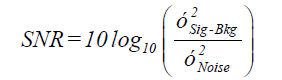
Where, Bkg=μNoise

Figure 3: Schematic representation of the areas used to calculate SNR.
Matching detected cells to ground truth cells
Ground truth cells were identified by manually reviewing each video file, and providing for each such cell the location and frame(s) in which it occurs. The cells were annotated while crossing the frames using a MATLAB application developed to assist with this task (Figure 4).

Figure 4: Two ground truth cells identified in the frame. The cells were annotated and X,Y coordinates (beginning and the end point of the cell) are recorded.
In order to facilitate the automatic evaluation of various cell detection/identification algorithms, we developed a MATLAB application for matching the detected cells to the ground truth cells. First, a complete weighted bipartite graph is built having as vertices all of the detected cells ‘D’ and all the ground–truth cells ‘T’ in all the video frames (Figure 5a), and edges between (D, T) with weight equal to the minimum (across all the frames where both cells appear) of the distance between the bounding boxes (in the same frame) of the cells corresponding to ‘D’ and ‘T’ (Figure 5b). Next, we remove all edges with weight above a user provided threshold, and replace the edge weights w(D, T) with wmax − w(D, T), where wmax is the maximum edge weight (Figure 5c). Finally, we compute a maximum weight matching in the resulting graph.

Figure 5: (a) Complete weighted bipartite graph using the distance as weight.(b) Minimal weigh is used to match Detected and True cells. (c) Using a user defined threshold, all the weights above the threshold (in this case distance of 2) are removed and the matched cells are classified as TP, the unmatched true cells are classified as FN and the unmatched detected cells are classified as FP.
This matching associates each detected cell with at most ground truth cell. Note that some detected cells may not be matched with any ground truth cell; in which case, we consider such detected cells as “false positives” (FP). Similarly, some ground truth cells may not be matched with any detected cell; in which case, we consider such ground truth cells as “false negatives” (FN). The matched detected cells are considered “true positives” (TP).
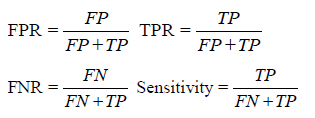
Upon counting the FN, FP, and TP cells, we calculate the false positive rate (FPR), false negative rate (FNR), true positive rate (TPR) and sensitivity as showed below:
Performance of our In-House method compared with current methodology for cell tracking
We compare the performance of our method with CellTrack (edge detection method) and MTrack2 (standard thresholding method). We feed the same frame sequences to these tools and compared the results with our algorithm (Figure 6). CellTrack requires inputting the initial edge threshold and the edge linking threshold for efficient edge detection. We set the initial edge threshold between 30-60, and we set the edge linking threshold between 20-50 for all the samples. For MTrack2, the threshold for detection was set between 140-150 and the minimal size object detected was 20 pixels.

Figure 6: Screenshot of MTrack2 (right) and CellTrack (left) for the same frame. CellTrack partially detected the cell on the right, but miss a fainter cell on the left. MTrack2 did a better job detecting both cells.
Results
Our algorithm along with Mtrack2 and CellTrack were evaluated in video files from all the 27 samples containing 1 cell/mL. Tables 1 and 2 show the detection results of our algorithm, MTrack2 and CellTrack respectively as compared with the ground truth. The samples are ordered by the average Signal-to-Noise Ratio (SNR) of their ground truth cells. The SNR of a cell is the maximum of the SNR’s of all of its occurrences (Table 3).
| ID | FP | FN | TP | GT | FPR | FNR | TPR | Sensitivity | SNR |
|---|---|---|---|---|---|---|---|---|---|
| 27 | 2 | 8 | 12 | 20 | 0.14 | 0.4 | 0.86 | 0.6 | 2.86 |
| 28 | 1 | 8 | 22 | 30 | 0.04 | 0.27 | 0.96 | 0.73 | 3.03 |
| 35 | 3 | 17 | 13 | 30 | 0.19 | 0.57 | 0.81 | 0.43 | 3.41 |
| 34 | 6 | 22 | 7 | 29 | 0.46 | 0.76 | 0.54 | 0.24 | 3.42 |
| 32 | 0 | 10 | 13 | 23 | 0 | 0.43 | 1 | 0.57 | 3.5 |
| 31 | 3 | 10 | 19 | 29 | 0.14 | 0.34 | 0.86 | 0.66 | 3.55 |
| 29 | 1 | 14 | 16 | 30 | 0.06 | 0.47 | 0.94 | 0.53 | 3.71 |
| 23 | 4 | 6 | 28 | 34 | 0.13 | 0.18 | 0.88 | 0.82 | 4.05 |
| 26 | 2 | 11 | 26 | 37 | 0.07 | 0.3 | 0.93 | 0.7 | 4.08 |
| 30 | 1 | 14 | 11 | 25 | 0.08 | 0.56 | 0.92 | 0.44 | 4.15 |
| 33 | 0 | 8 | 17 | 25 | 0 | 0.32 | 1 | 0.68 | 4.27 |
| 24 | 5 | 2 | 27 | 29 | 0.16 | 0.07 | 0.84 | 0.93 | 4.41 |
| 17 | 4 | 4 | 20 | 24 | 0.17 | 0.17 | 0.83 | 0.83 | 4.52 |
| 25 | 1 | 4 | 29 | 33 | 0.03 | 0.12 | 0.97 | 0.88 | 4.56 |
| 22 | 1 | 3 | 24 | 27 | 0.04 | 0.11 | 0.96 | 0.89 | 4.58 |
| 15 | 1 | 1 | 22 | 23 | 0.04 | 0.04 | 0.96 | 0.96 | 4.64 |
| 20 | 1 | 5 | 26 | 31 | 0.04 | 0.16 | 0.96 | 0.84 | 5.02 |
| 21 | 3 | 3 | 18 | 21 | 0.14 | 0.14 | 0.86 | 0.86 | 5.08 |
| 19 | 2 | 4 | 25 | 29 | 0.07 | 0.14 | 0.93 | 0.86 | 5.09 |
| 18 | 1 | 3 | 28 | 31 | 0.03 | 0.1 | 0.97 | 0.9 | 5.37 |
| 13 | 1 | 3 | 27 | 30 | 0.04 | 0.1 | 1.96 | 0.9 | 5.91 |
| 12 | 4 | 0 | 21 | 21 | 0.16 | 0 | 0.84 | 1 | 6.02 |
| 16 | 0 | 1 | 20 | 21 | 0 | 0.05 | 1 | 0.95 | 6.2 |
| 14 | 0 | 1 | 30 | 31 | 0 | 0.03 | 1 | 0.97 | 6.25 |
| 11 | 2 | 1 | 25 | 26 | 0.07 | 0.04 | 0.93 | 0.96 | 6.46 |
| 9 | 1 | 3 | 24 | 27 | 0.04 | 0.11 | 0.96 | 0.89 | 7.42 |
| 10 | 2 | 1 | 24 | 25 | 0.08 | 0.04 | 0.92 | 0.96 | 7.44 |
ID=cell number; FP=False Positive; FN= False negative; TP=True Positive; FPR False Positive Rate; FNR=False Negative Rate; TPR=True Positive Rate; GT=Ground Truth Cells.
Table 1: Detection performance of our method. Samples sorted by the average SNR of their ground truth cells.
| ID | FP | FN | TP | GT | FPR | FNR | TPR | Sensitivity | SNR |
|---|---|---|---|---|---|---|---|---|---|
| 27 | 22 | 17 | 3 | 20 | 0.88 | 0.85 | 0.12 | 0.15 | 2.86 |
| 28 | 22 | 16 | 12 | 28 | 0.65 | 0.57 | 0.35 | 0.43 | 3.03 |
| 35 | 52 | 18 | 12 | 30 | 0.81 | 0.6 | 0.19 | 0.4 | 3.41 |
| 34 | 7 | 23 | 6 | 29 | 0.54 | 0.79 | 0.46 | 0.21 | 3.42 |
| 32 | 162 | 9 | 14 | 23 | 0.92 | 0.39 | 0.08 | 0.61 | 3.5 |
| 31 | 24 | 21 | 8 | 29 | 0.75 | 0.72 | 0.25 | 0.28 | 3.55 |
| 29 | 34 | 23 | 7 | 30 | 0.83 | 0.77 | 0.17 | 0.23 | 3.71 |
| 23 | 63 | 6 | 28 | 34 | 0.69 | 0.18 | 0.31 | 0.82 | 4.05 |
| 26 | 37 | 18 | 19 | 37 | 0.66 | 0.49 | 0.34 | 0.51 | 4.08 |
| 30 | 77 | 11 | 14 | 25 | 0.85 | 0.44 | 0.15 | 0.56 | 4.15 |
| 33 | 11 | 12 | 13 | 25 | 0.46 | 0.48 | 0.54 | 0.52 | 4.27 |
| 24 | 5 | 18 | 11 | 29 | 0.31 | 0.62 | 0.69 | 0.38 | 4.41 |
| 17 | 0 | 8 | 16 | 24 | 0 | 0.33 | 1 | 0.67 | 4.52 |
| 25 | 37 | 9 | 24 | 33 | 0.61 | 0.27 | 0.39 | 0.73 | 4.56 |
| 22 | 26 | 14 | 13 | 27 | 0.67 | 0.52 | 0.33 | 0.48 | 4.58 |
| 15 | 0 | 10 | 13 | 23 | 0 | 0.43 | 1 | 0.57 | 4.64 |
| 20 | 12 | 17 | 14 | 61 | 0.46 | 0.55 | 0.54 | 0.45 | 5.02 |
| 21 | 13 | 10 | 11 | 21 | 0.54 | 0.48 | 0.46 | 0.52 | 2.08 |
| 19 | 12 | 15 | 14 | 29 | 0.46 | 0.52 | 0.54 | 0.48 | 5.09 |
| 18 | 4 | 6 | 25 | 31 | 0.14 | 0.19 | 0.86 | 0.81 | 5.37 |
| 13 | 0 | 1 | 29 | 30 | 0 | 0.03 | 1 | 0.97 | 5.91 |
| 12 | 0 | 2 | 19 | 21 | 0 | 0.1 | 1 | 0.9 | 6.02 |
| 16 | 0 | 5 | 16 | 21 | 0 | 0.24 | 1 | 0.76 | 6.2 |
| 14 | 0 | 7 | 24 | 31 | 0 | 0.23 | 1 | 0.77 | 6.25 |
| 11 | 0 | 0 | 26 | 26 | 0 | 0 | 1 | 1 | 6.46 |
| 9 | 1 | 3 | 24 | 27 | 0.04 | 0.11 | 0.96 | 0.89 | 7.42 |
| 10 | 0 | 2 | 23 | 25 | 0 | 0.08 | 1 | 0.92 | 7.44 |
Table 2: MTrack2 results.
| ID | FP | FN | TP | GT | FPR | FNR | TPR | Sensitivity | SNR |
|---|---|---|---|---|---|---|---|---|---|
| 27 | 29 | 15 | 5 | 20 | 0.85 | 0.75 | 0.15 | 0.25 | 2.86 |
| 28 | 99 | 27 | 1 | 28 | 0.99 | 0.96 | 0.01 | 0.04 | 3.03 |
| 35 | 34 | 24 | 6 | 30 | 0.85 | 0.8 | 0.15 | 0.2 | 3.41 |
| 34 | 50 | 23 | 6 | 29 | 0.89 | 0.79 | 0.11 | 0.21 | 3.42 |
| 32 | 11 | 22 | 1 | 23 | 0.92 | 0.96 | 0.08 | 0.04 | 3.5 |
| 31 | 19 | 21 | 8 | 29 | 0.7 | 0.72 | 0.3 | 0.28 | 3.55 |
| 29 | 29 | 16 | 14 | 30 | 0.67 | 0.53 | 0.33 | 0.47 | 3.71 |
| 23 | 23 | 23 | 11 | 34 | 0.68 | 0.68 | 0.32 | 0.32 | 4.05 |
| 26 | 40 | 18 | 19 | 37 | 0.68 | 0.49 | 0.32 | 0.51 | 4.08 |
| 30 | 33 | 16 | 9 | 25 | 0.79 | 0.64 | 0.21 | 0.36 | 4.15 |
| 33 | 21 | 21 | 4 | 25 | 0.84 | 0.84 | 0.16 | 0.16 | 4.27 |
| 24 | 47 | 22 | 7 | 29 | 0.87 | 0.76 | 0.13 | 0.24 | 4.41 |
| 17 | 50 | 6 | 18 | 24 | 0.74 | 0.25 | 0.26 | 0.75 | 4.52 |
| 25 | 39 | 3 | 20 | 33 | 0.66 | 0.39 | 0.34 | 0.61 | 4.56 |
| 22 | 62 | 24 | 3 | 27 | 0.95 | 0.89 | 0.05 | 0.11 | 4.58 |
| 15 | 73 | 10 | 13 | 23 | 0.5 | 0.43 | 0.15 | 0.57 | 4.64 |
| 20 | 70 | 15 | 16 | 31 | 0.81 | 0.48 | 0.19 | 0.52 | 5.02 |
| 21 | 91 | 8 | 13 | 21 | 0.88 | 0.38 | 0.13 | 0.62 | 5.08 |
| 19 | 44 | 12 | 17 | 29 | 0.72 | 0.41 | 0.28 | 0.59 | 5.09 |
| 18 | 37 | 22 | 9 | 31 | 0.8 | 0.71 | 0.2 | 0.29 | 5.37 |
| 13 | 26 | 14 | 16 | 30 | 0.62 | 0.47 | 0.38 | 0.53 | 5.91 |
| 12 | 73 | 8 | 13 | 21 | 0.85 | 0.38 | 0.15 | 0.62 | 6.02 |
| 16 | 36 | 10 | 11 | 21 | 0.77 | 0.48 | 0.23 | 0.52 | 6.2 |
| 14 | 60 | 2 | 29 | 31 | 0.67 | 0.06 | 0.33 | 0.94 | 6.25 |
| 11 | 26 | 3 | 23 | 26 | 0.53 | 0.12 | 0.47 | 0.88 | 6.46 |
| 9 | 6 | 3 | 24 | 27 | 0.2 | 0.11 | 0.8 | 0.89 | 7.42 |
| 10 | 14 | 1 | 24 | 25 | 0.37 | 0.04 | 0.63 | 0.96 | 7.44 |
Table 3: CellTrack results.
The average sensitivity for samples with SNR ≥ 4.4 dB, is 91% for our method, 71% for MTrack2 and 60% for CellTrack (Table 4), while across all samples is 78%, 59% and 46% for our method, MTrack2, and CellTrack respectively (Table 5).
| FPR | FNR | TPR | Sensitivity | |
|---|---|---|---|---|
| CellTrack | 0.71 | 0.4 | 0.29 | 0.6 |
| MTrack2 | 0.2 | 0.29 | 0.8 | 0.71 |
| In-House | 0.07 | 0.09 | 0.93 | 0.91 |
Table 4: Performance comparison of our algorithm versus MTrack2 and CellTrack for samples with (SNR ≥4.4dB).
| FPR | FNR | TPR | Sensitivity | |
|---|---|---|---|---|
| CellTrack | 0.75 | 0.54 | 0.25 | 0.46 |
| MTrack2 | 0.42 | 0.41 | 0.58 | 0.59 |
| In-House | 0.09 | 0.22 | 0.91 | 0.78 |
Table 5: In-house algorithm compared with MTrack2 and CellTrack (All SNRs values).
Our algorithm performs better than CellTrack and MTrack2 for all the samples as well as the samples with SNR at least 4.4 dB. In addition, the average value for false positive and false negative rates were considerably smaller in our algorithm (0.07 and 0.09 respectively) compared with MTrack2 and CellTrack (Table 4).
Considering all SNRs values across all samples, our algorithm also performed better than MTrack2 and CellTrack (Table 5).
Figure 7 shows a scatterplot of all the samples (with NSR at least 4.4 dB) arranged by the sensitivity achieved by the various methods. We can clearly see that our algorithm shows substantially better (and never worse) sensitivity for all the samples as compared with MTrack2 and CellTrack.

Figure 7: Scatterplot representing samples arranged by sensitivity for samples with SNR equal or greater than 4.41 dB comparing our in-house procedure with MTrack2 and CellTrack. Notice all the Blue circles (our method) are always above the 0.80 mark.
Conclusion
Our algorithm performed better than current methods for cell detection and enumeration (average true positive rate of 93% TPR and sensitivity of 91%) in detection of cells in concentrations of 1 cell/ml for samples with SNR at least 4.4 dB. In comparison, current commonly- -used edge detection or threshold based tools such CellTrack and MTrack2 did not performed well. CellTrack (based on Canny-style edge detection) fails to detect faint moving streaks in the moving background producing a high false positive rate. MTrack2 (based on a thresholding method) performs better than CellTrack but still much worse than our method.
Our method enables automation of the new imaging cytometry technique for rare cell detection. Wide field video imaging cytometry combined with cell streak imaging results in a simpler, affordable, and more portable flow cytometer, which facilitates the expansion of cellbased clinical diagnostics, especially in resource-poor settings.
For samples with SNR lower than 4.4 dB, our algorithm was able to detect only ~58% of the true cells. Our algorithm for cell detection relies in part on the ability to differentiate cells from noise in each individual frame, therefore the algorithm performed poorly for very faint cells. In order to detect these faint cells other techniques based on recognition of pixel spatial patterns and expected location in the frame may be used. In future research we plan to develop a methodology for detecting rare cells with lower SNR values.
Appendix
Automated streak detection and counting algorithm
Streak detection and binary mask: The objective of this procedure is to create a binary mask with the location of all the streaks in the frames that potentially represent cells. The creation of the binary mask is achieved through the procedure I “ComputeStreakMask”. The major steps of this procedure (in MATLAB-like pseudocode) are given below.
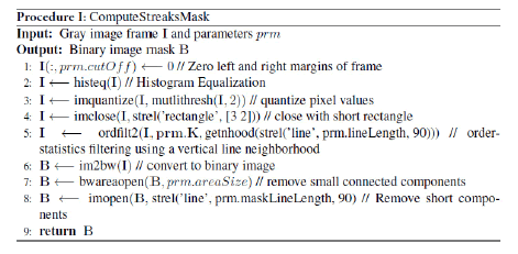
Step 1: The 640 × 480 pixel frames are preprocessed by removing 40 pixels in left and right margins to eliminate artifacts showed in the margins of the frame (Figure 8a).

Figure 8: Frame processing from step 1 to 4 (Procedure I). Notice in (c), the streaks are hidden by high noise generated by the procedure to fill small gaps along the boundary of foreground objects.
Steps 2-3: The image intensity is adjusted by histogram equalization, then two thresholds values (of the image intensity) are selected using Otsu’s method quantizing the image into three levels (Figure 8b).
Step 4: In order to fill small gaps along the boundary of foreground objects, a morphological close with a 3 × 2 pixels rectangle is slide across each frame. This procedure generates unwanted noise (Figure 8c), but the foreground objects (potential streaks) become more defined (no gaps along the boundary).
Step 5: In order to reduce the background noise generated in the previous steps, a 2D order statistic filtering is performed. Briefly, a 23 × 1 pixels rectangle is slid across the frame, replacing the pixel value at the rectangle origins with the 3rd smallest of the pixel contained in the rectangle. The result of this operation will eliminate pixels with low values around the foreground object, but will preserve pixels with small values inside the foreground object (Figures 9a and 9b).

Figure 9: Step 5, 6, Procedure I. (a) resulting high noise image from the previous step. (b) 2D order filtering was used to reduce background noise and (c) the three-level image is converted to a binary image (c).
Step 6: The three level threshold image is converted to a binary image (Figure 9c).
Steps 7, 8: This steps are necessary to clean the image from small artifacts and eliminate extrusions from the boundary of foreground objects. All objects (potential streaks) smaller than 50 pixels are eliminated (Figures 10a and 10b), then, a morphological open, with an 81 × 1 rectangle, is performed to remove non-vertical short objects, this objects most probably represent artifacts. The final result of this procedure is a binary mask with the location of all the streaks that potential represent cells (Figure 10c).

Figure 10: All the foreground objects smaller than 50 pixels a long with non-vertical short objects are discarded. In addition, all the extrusion of the boundary of foreground objects are eliminated providing clean, well defined streaks mask(c). Notice, the binary mask (c) includes three streaks, but only the streak in the middle corresponds to a real cell.
Identifying candidate cells: The goal of this step is to identify all potential cells (candidate cells) using the streak location from the binary mask. This is achieved through procedure II “ComputeStreakAndCandidateCells”.
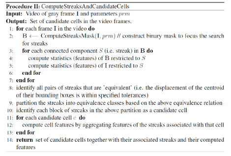
The binary mask from the previous step is overlaid with the original image and the streaks representing potential cells are enclosed in boundary boxes for further possessing (Figure 11). The following features are computed for each streak: (a) area, (b) bounding box (centroid, height, and width), (c) major and minor axes length of enclosed ellipsoid, (d) eccentricity, (e) orientation, (f) perimeter, and (g) descriptive statistics (min, max, media, quantiles, variance, sum) of the values of the streak’s pixels. Most of these features are provide by the “regionprops” MATLAB command. Streaks (across all frames) are grouped and labeled as equivalent if they are expected to belong to the same cell, based on the displacement of their centroids within a tolerance level. The streaks that are in the same equivalence class are now identified as a candidate cell. For each candidate cell, we compute aggregates (min, max, mean, median, range, variance) of the features of its streaks. Note that in MATLAB’s image coordinate system, the x-axis (y-axis) runs along the image’s width (height), increasing from left-toright (top-to-bottom) with the (0, 0) point at the upper-and–left–most pixel. By the end of this step the streaks are annotated and candidate cells are identified for each frame.

Figure 11: Overlaying the binary mask with the original image. Based in the binary mask, three objects are identified and classified as candidate cells (green lines) in the original frame.
Filtering out spurious cells and identifying true cells: The candidate cells identified in the previous steps are evaluated according to intensity and length. the goal of this procedure is to eliminate the cells with a low probability of being real cells. The major steps of this procedure are listed below (Procedure III).
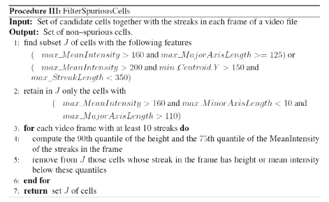
Briefly, to eliminate spurious cells, we computed the 90th quantile of streak height and 75th quantile of the streak mean intensity and we eliminated all the streaks in the frame with height or mean intensity below these values (Figure 12).

Figure 12: Eliminating Spurious cells. Only one object was classified as nonspurious cell(b) from the three objects identified in the previous steps (a).
References
- Allard WJ, Matera J, Miller MC, Repollet M, Connelly MC, Rao C, et al. (2004) Tumor cells circulate in the peripheral blood of all major carcinomas but not in healthy subjects or patients with nonmalignant diseases. Clin Cancer Res 10: 6897-904.
- de Wit S, van Dalum G, Terstappen LW (2014) Detection of circulating tumor cells. Scientifica (Cairo) 2014: 819362.
- Giuliano M,Giordano A, Jackson S, De Giorgi U, Mego M, et al.(2014) Circulating tumor cells as early predictors of metastatic spread in breast cancer patients with limited metastatic dissemination. Breast Cancer Research,p: 16.
- Alix-Panabieres C, Pantel K (2012) Circulating Tumor Cells: Liquid Biopsy of Cancer. Clinical Chemistry 59: 110-118.
- Li P,Zackary S, Stratton S, Ming D, Ritz J, et al. (2013) Probing circulating tumor cells in microfluidics. Lab on a Chip 13: 602.
- Chang CL,Huang W, Jalal SI, Chan BD, Mahmood A, et al. (2015) Circulating tumor cell detection using a parallel flow micro-aperture chip system. Lab on a Chip15: 1677-1688.
- Golden JP, Kim JS, Erickson JS, Hilliard LR, Howell PB,et al. (2009) Multi-wavelength microflow cytometer using groove-generated sheath flow. Lab on a Chip 9: 1942.
- Howell Jr PB,Golden JP, Hilliard LR, Erickson JS, Mott DR, et al. (2008) Two simple and rugged designs for creating microfluidic sheath flow. Lab on a Chip 8: 1097.
- Zuba-Surma EK, Ratajczak MZ (2011) Analytical Capabilities of the ImageStream Cytometer. Methods in Cell Biology, Elsevier BV, pp: 207-230.
- Ngundi MM, Qadri SA, Wallace EV, Moore MH, Lassman ME,et al. (2006) Detection of Deoxynivalenol in Foods and Indoor Air Using an Array Biosensor. Environmental Science & Technology 40: 2352-2356.
- Sun S, Francis J, Sapsford KE, Kostov Y, Rasooly A (2010) Multi-wavelength spatial LED illumination based detector for in vitro detection of botulinum neurotoxin A activity. Sensors and Actuators B: Chemical 146: 297-306.
- Sun S, Ossandon M, Kostov Y, Rasooly A (2009) Lab-on-a-chip for botulinum neurotoxin a (BoNT-A) activity analysis. Lab on a Chip 9: 3275.
- Navruz I, Coskun AF, Wong J, Mohammad S, Tseng D, Nagi R, et al. (2013) Smart-phone based computational microscopy using multi-frame contact imaging on a fiber-optic array. Lab on a Chip 13: 4015.
- Wei Q, Qi H, Luo W, Tseng D, Ki SJ,et al. (2013) Fluorescent Imaging of Single Nanoparticles and Viruses on a Smart Phone. ACS Nano 7: 9147-9155.
- Zhu H, Ozcan A (2013) Wide-field Fluorescent Microscopy and Fluorescent Imaging Flow Cytometry on a Cell-phone. Journal of Visualized Experiments, p: 74.
- Balsam J, Bruck HA, Rasooly A (2014) Webcam-based flow cytometer using wide-field imaging for low cell number detection at high throughput. The Analyst 139:4322.
- Balsam J, Bruck HA, Rasooly A (2015) Cell streak imaging cytometry for rare cell detection. Biosensors and Bioelectronics 64: 154-160.
- Huth J, Buchholz M, Kraus JM, M�?¸lhave K, Gradinaru C,et al. (2011) TimeLapseAnalyzer: Multi-target analysis for live-cell imaging and time-lapse microscopy. Computer Methods and Programs in Biomedicine 104: 227-234.
- Lamprecht M, Sabatini D, Carpenter A (2007) CellProfilerâ�?¢: free, versatile software for automated biological image analysis. BioTechniques 42: 71-75.
- Sacan A, Ferhatosmanoglu H,Coskun H (2008) CellTrack: an open-source software for cell tracking and motility analysis. Bioinformatics 24: 1647-1649.
- Shen H, Nelson G, Kennedy S, Nelson D, Johnson J,et al. (2006) Automatic tracking of biological cells and compartments using particle filters and active contours. Chemometrics and Intelligent Laboratory Systems 82: 276-282.
- Hand AJ, Sun T, Barber DC, Hose DR, MacNeil S (2009) Automated tracking of migrating cells in phase-contrast video microscopy sequences using image registration. Journal of Microscopy 234: 62-79.
- Meijering E, Dzyubachyk O, Smal I (2012) Methods for Cell and Particle Tracking, in Imaging and Spectroscopic Analysis of Living Cells - Optical and Spectroscopic Techniques. Elsevier BV,pp: 183-200.
- Sankur B (2004) Survey over image thresholding techniques and quantitative performance evaluation. J Electron Imaging 13: 146.
- Ossandon M (2017) A computational streak mode cytometry biosensor for rare cell analysis. Analyst.
- Otsu N (1979) A Threshold Selection Method from Gray-Level Histograms. IEEE Transactions on Systems, Man and Cybernetics 9: 62-66.
Relevant Topics
Recommended Journals
Article Tools
Article Usage
- Total views: 9286
- [From(publication date):
June-2017 - Aug 25, 2025] - Breakdown by view type
- HTML page views : 8254
- PDF downloads : 1032