Issues Related to the Use of One-dimensional Ocean-diffusion Models for Determining Climate Sensitivity

Study of the Earth’s climate can utilize a variety of investigative tools. They include observations through a multitude of instruments such as land-based temperature sensors or remote sensing systems such as those on Earth-observing satellites. Other sensors include oceanographic measurement devices such as the Argo float or the expendable bathythermograph [1]. Deep-time measurements can be obtained from proxy information from ice cores, tree rings, sediments, and other natural archives.

Another principal set of tools for climate science are climate models which are computer simulations that employ conservation of mass, momentum, and energy and thermodynamic analysis to predict future climate states. Computer simulations vary in complexity from zero-dimensional versions which treat the Earth system as a single homogeneous entity, to very complex three-dimensional General Circulation Models (GCM) which simulate the flow of the atmosphere and the oceans and their interaction with each other. GCMs are computationally expensive ventures and require large-capacity supercomputers with massive multi-parallel computer architecture and large storage capacity. Consequently, their employment is limited to major research institutions.

Alternatives to very simplistic zero-dimensional models and highly-complex GCMs are models of intermediate complexity. They may be one- or two-dimensional models that include the atmosphere or the ocean, or both. While intermediate models are not able to fully capture the spatial variation of the Earth’s climate, they can be used to quickly estimate the impact of various processes.

Despite their simplicity, it is important that the downscaled intermediate models represent physical phenomena and provide realistic results. Furthermore, sound numerical methodology must be used to ensure results of high veracity.

In this study, we explore a simple one-dimensional ocean diffusion model, previously published by Spencer and Braswell [2] (hereafter SB14) as a case study of the issues that must be addressed for proper calculations. Here, the ocean is treated as a uniform water body that covers the globe. No horizontal flow of energy is allowed in this simple model, only vertical diffusion of heat can occur. SB14 explored three different scenarios. In the first scenario, only human and volcanic impacts were included (human caused global warming and cooling effects which followed volcanic eruptions). The second model incorporated the first study with the addition of non-radiative internal variability (essentially internal variability in the climate associated with ocean mixing). Finally, the third model encompassed the second with the addition of an extra term associated with a change in energy inputs to the oceans from cloud formation, which they called “Internal Radiative Forcing” (IRF). The conclusion made by the authors is that the canonical sensitivity of the Earth’s climate to increasing greenhouse gases is significantly overestimated by models (including GCMs) that fail to include their IRF term. If these conclusions are true, it would overturn decades of established climate science and invalidate most current state of the art climate models.

The use of simple ocean models in itself is not novel. In fact, there is a rich body of literature that has developed on this topic. Among the originators of diffusion simulations of the Earth’s oceans are [3] and [4]. The motivation of these studies was to quantify diffusion of carbon dioxide in the ocean depths. Even by 1983 however, there was recognition that the ocean was not merely diffusive but rather includes important flows of water that redistribute heat (advection). For the oceans, surface currents flow from the equator to the poles where they sink to the ocean depths and spread across the globe. This understanding led to the development of advection-diffusion models which added water flow to the energy transport equations [5-9].

A schematic of the typical treatment of advection-diffusion is provided in Figure 1. It should be recognized that the figure shows one manifestation of the model. Other versions include water transfer between the main ocean zone and the Polar Regions at intermediate depths.

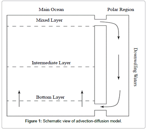
Figure 1: Schematic view of advection-diffusion model.

A diffusion only model is expressed mathematically as

(1)

where the symbols ρ, c, and k are the density, heat capacity, and thermal conductivity of the water. The symbol T can represent the temperature or a temperature anomaly (temperature excursion from some undisturbed value), depending on the desired output of the model. The conductivity is located inside a differential operator on the right hand side to reflect the possibility it is a spatially varying quantity. It is common to recast Equation (1) as

(2)

where α is the thermal diffusivity.

When advection is included, Equation (2) becomes

(3)

where w is the vertical advection velocity. The sign of the right-most term is positive or negative depending on whether the vertical velocity is defined positively upwards or downwards. It can be seen that the inclusion of advection incorporates a term that is proportional to the temperature gradient (in addition to the diffusion term). The thermal diffusivity α will be allowed to be dependent on the depth.

Detailed development of the diffusion-only mathematical model

The methodology followed here will be based on the diffusion-only approach applied to a series of control volumes which subdivide the ocean column; it is based on the SB14 approach. The control volumes are set to 50 m depths and extend to 2000 m. There are, therefore, 40 volumes which constitute the column. The volumes are numbered 1, 2,….40 where 1 represents the surface element. The diffusion equation (Equation (1)) from SB14 is repeated here as it is to be applied to the surface element. There is now an inclusion of ocean mixing and radiative heating and cooling associated with cloud variations. The new expression is

(4)

The subscript 1 refers to the element over which the equation is applied. The term N(t) represents all radiation forcings (internal and external) at the surface, λT₁ is the radiative feedback (increase ocean surface temperature which causes heat loss). The last term, S₁ is nonradiative energy changes associated with ocean mixing, although no mention of turbulent fluxes was provided. The symbol C_p represents the heat capacity of a control volume thick layer of ocean water.

It is seen that in Equation (4), the thermal diffusivity has been placed outside of the differential operator by SB14. Such a move is permissible only when the diffusivity is uniform; however, for the present case, it produces an error that will be quantified later. In the following equations, which are also taken from SB14, this error has been repeated.

For layers 2, 3, and 4, the governing equations are:

(5)

The inclusion of the mixing term S_i allows energy exchange between the layers which constitute the upper 200 meters of the ocean column.

Finally, for layers i > 4,

(6)

It should be noted that the approach shown here, which is reproduced from SB14, allows the thermal diffusivity at each layer to be specified independently. From a practical standpoint, the diffusivities for layers 6 and deeper are set equal to each other.

To complete the model development, information about N and S must be provided. Both terms are set to be proportional to the Multivariate ENSO Index (MEI), which is a measure of El Nino activity in the Pacific Ocean. The constants of proportionality are tunable parameters.

In total, the model provided here (taken from SB14) includes ten tunable parameters. The selection of the resulting tunable parameters was based on a comparison of the model results with ocean temperature information from Levitus [10].

In terms of the model outcome, the resulting feedback parameter λ represents the amount of heat flow which will cause a 1°C global temperature rise. Units of λ are heat flux per degree (W/m² °C). The importance of λ is that its inverse is used to determine the climate sensitivity, which has units of °C/(W/m²).

It should also be noted that another concern with the model is that it ignores approximately 30% of the global surface (area covered by land). Consequently, the resulting feedback parameter, even if the model is executed correctly, will be too large (and the resulting climate sensitivity will be too small).

In addition, the proposed model of SB14 incorporates a globally uniform El Nino forcing. Even though the El Nino process is limited to a small region in the Pacific Ocean, it certainly has a global impact on the atmosphere. However, assigning ocean diffusion terms uniformly across the globe based on phenomena in a very small geographic region is highly questionable. Finally, the model ignores latent heat exchange between the ocean and the atmosphere (heat transfer associated with evaporation of ocean water at the surface and condensation within the atmosphere). Latent heat transfer, which is a spatially non-uniform effect, can be large in some regions of the globe.

The numerical method

Solution of Equations (4-6) requires application of the equations to the control volumes which were already described. To aid the discussion, a nomenclature describing diffusive heat transfer between three points (North, Point, South) are shown embedded within Figure 2. This nomenclature is taken from the seminal numerical methods text by [11]. The image shows energy entering heat from the upper boundary (labeled n). Heat leaves the bottom through boundary s.

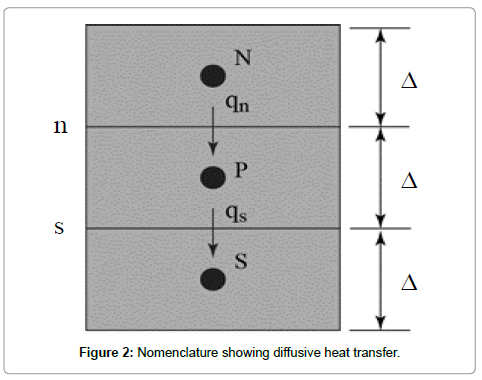
Figure 2: Nomenclature showing diffusive heat transfer.

The diffusive equation, when applied to element P and with the neglect of surface mixing is

(7)

Here, the timewise integration is performed explicitly such that all transfer terms are evaluated at the previous (old) timestep. Other options include fully implicit (all transfer terms evaluated using new temperature) and the Crank-Nicholson scheme (which evaluates heat transfer terms at both the previous and current temperatures and then uses an average value). The explicit method, which is used here, is unique in that it is not unconditionally stable; the time step must satisfy the following criteria to avoid instability (Equation (8)). On the other hand, its simplicity is an advantage. The explicit method was used in SB14 and will be employed here as well.

(8)

It should be noted that a proper numerical simulation should demonstrate both mesh and time-step independence. It is not clear that this step was completed by SB14. The purpose of the present study is to highlight errors in the underlying methodology of SB14. Consequently, the choice of SB14 timesteps and mesh size are repeated here without alteration. Further study on whether their timesteps and element sizes are sufficient could be carried out in the future. Separate calculations have shown that the numerical method used by SB14 is, in fact, unstable for certain values of diffusivity.

A frequent error in diffusive calculations (and an error in SB14) relates to the appropriate thermal diffusivity values. Lowercase n and s are used to symbolize the interface above and below the central element P. The diffusivity associated with the upper energy flow is α_n and the counterpart for the lower flow is αs. These diffusivities are not associated with any particular element (as assumed in SB14). Rather they must characterize an average diffusivity at an interface. It has been shown [11] that the correct diffusivity is the harmonic mean of adjoining elements so that

(9)

Here, the subscripts P and N denote thicknesses of the upper and central elements, respectively. The correct method, which combines Equations (7) and (9) can be compared with the approach taken in SB14. In the SB14 manuscript, the energy equation for layer i utilized only the diffusivity for that layer, as evident in Equations (5) and (6). On the other hand, the programming code graciously provided by the SB14 authors actually employed a different procedure. There, they used the upstream diffusivity to calculate a downstream heat flow. Therefore, heat flow qn was calculated using α_N and heat flow qs was calculated using α_P. In the following, the approach actually used in the SB14 calculations will be adopted. That approach leads to

(10)

Comparison of Equation (10) with (7) reveals two errors. First, the diffusivity was evaluated asymmetrically with respect to the interface through which heat transfer occurs. Second, the diffusivity values were taken to be those of the elements themselves rather than the harmonic mean of adjacent cells.

Boundary conditions

Another major issue to be addressed is the treatment of boundary elements (i=1 and 40). First, attention is turned to the surface element. The development of the numerical approach must provide the surface temperature of the ocean waters because this temperature is responsible for radiative exchange [11,12]. With this recognized it is seen that Equation (4), as utilized by SB14 should, in fact, be written as

(11)

where T_surf signifies the water surface temperature. A number of alternative approaches are available to allow calculation of both T₁ and T_surf and will now be described.

The first option, which is shown in Figure 3, is most commonly employed for its simplicity. This method is universally recommended in all heat transfer undergraduate textbooks for example. From the figure, it is seen that the surface element is half the size of an interior cell. The calculation node is thereby positioned on the surface so T1 and Tsurf are coincident. If this approach is employed, the thermal inertia term must be divided by 2.

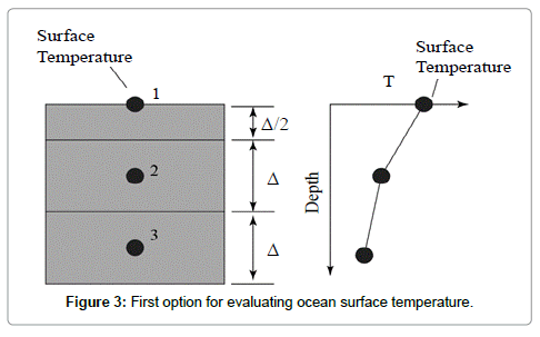
Figure 3: First option for evaluating ocean surface temperature.

A second option is to position a very thin element at the surface as shown in Figure 4. With this approach, the equations of transfer must account for the non-uniform element thickness however it has an advantage of resulting in a higher density of calculation locations near the ocean surface which allows for some consideration of the near-surface processes that are known to be instrumental for air-sea interaction.

Figure 4: Second option for determining ocean surface temperature.

If, on the other hand, it is recognized that the upper layer of the ocean is characterized by extensive ocean currents which tend to homogenize the fluid temperature, a third alternative becomes possible. This third alternative, shown schematically in Figure 5, has annotations identifying the homogeneous mixed layer. If this approach is taken, then it is quickly seen that the diffusion of heat into element 2 occurs over a distance Δ/2 (rather than Δ). Mathematically, location 1’ should replace location 1 for the diffusion term in the difference equation.

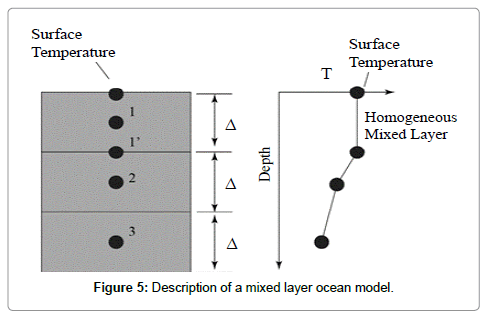
Figure 5: Description of a mixed layer ocean model.

With the preceding discussion as background, attention is turned to the practice actually employed in SB14. There, neither a true diffusion nor a mixed-layer were utilized. Rather, the temperature at node 1, which was positioned 25 meters beneath the ocean surface, was assigned to the surface. Schematically, this approach is shown in Figure 6. On the right-hand side of the figure, the temperature labeled “Incorrect Temperature” is that from SB14 and that labeled “Surface Temperature” is the correct result if a diffusion model is employed throughout the entire ocean column.

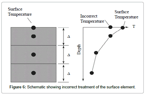
Figure 6: Schematic showing incorrect treatment of the surface element.

While the mathematical treatment showcased in Figures 3, 4, and 5 are correct, only Figure 5 accounts for the physically realistic mixed layer; consequently it will be employed here in a corrected diffusiononly ocean model. Notably, neither approach takes into account the surface skin layer, which is also fundamental to air-sea interaction and is therefore a caveat of even this approach.

Finally, attention is turned to the lowermost element in the water column. In SB14, this location was taken to be 2000 m. In the description provided within SB14, no mention is made of any special treatment for the bottom layer. However, examination of the computer program, generously provided by the authors of SB14, showed that the authors actually insulated the ocean bottom. The insulation impact is shown in Figure 7. Since no heat was allowed to flow through the bottom element, it means that, in effect, ocean layers below 2000 m have no heat capacity. Inasmuch as experiments clearly show significant heat has been detected beneath the 2000 m layer, this approach is inappropriate ([1] and references contained therein). In the correction to the SB14 to be presented shortly, the ocean waters will be simulated to 4000 m (80 layers).

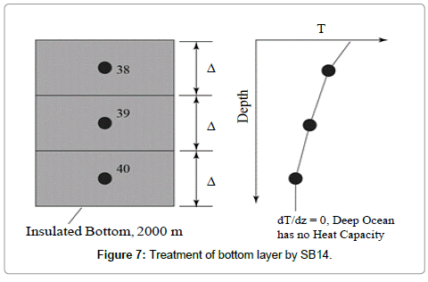
Figure 7: Treatment of bottom layer by SB14.

Summary of sources of error from simple one-dimensional diffusion ocean models

It is useful to summarize the major concerns with the modeling approach taken in SB14 and other similar studies. They are listed here in no particular order.

1. Full global ocean cover (actually, approximately 70% of the Earth’s surface is water covered)

2. Neglect of advective heat transfer

3. Asymmetric thermal diffusivity used in calculations of heat diffusion

4. Use of element-averaged thermal diffusivity for calculation of heat transfer

5. Incorrect treatment of surface boundary element

6. Incorrect treatment of bottom boundary element

7. The model assigns an ocean process (El Nino cycle) which covers a limited geographic region in the Pacific Ocean as a global phenomenon

8. The model neglects latent heat transfer between the atmosphere and the ocean surface

In order to rehabilitate the simplified one-dimensional diffusiononly approach, some corrections to the SB14 model will be made. The focus here is on the impacts of the numerical methodology. Consequently, correct treatment of the thermal diffusivity and the upper and lower elements will be made. At the surface, the technique outlined in Figure 5 will be used. At the ocean bottom, the waters will be extended to 4000 m to provide a more realistic depth. The impact of these changes on the temperature variations will now be given.

As indicated in the preceding section, only corrections to the numerical methodology of the simplified one-dimensional diffusion model will be implemented. The first set of results to be presented is the temporal temperature variation of the top-most ocean layer (0-50 m) from 1955 until present. Figure 8 has been prepared which shows the corrected and uncorrected comparisons. It should be noted that neither the corrected nor the uncorrected versions address the uncertainties in the originating data and consequently, the meaningfulness of this exercise is questionable, even if the calculations were performed correctly, as we have done here. The upper part of the Figure (part (a)) is taken directly from SB14. It can be seen in the original calculation shown in part (a), that the match between the simulated and measured upper-layer temperatures appeared to be very good. On the other hand, the corrected methodology shows that the match is actually poor. In fact, the rate of change of corrected surface temperatures is approximately 63% of the measured values.

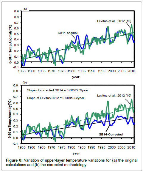
Figure 8: Variation of upper-layer temperature variations for (a) the original calculations and (b) the corrected methodology.

The impact of the corrected methodology extends beyond the upper layer. To showcase the results at deeper layers, Figure 9 has been prepared. That figure has been extended to 1000 meters to show a comparison of SB14 with [10]. The upper figure is taken from the SB14 and the lower part shows the impact of correct methodology on the results. It is seen that over the entire range of ocean measurements, the temperature increase from SB14 is significantly less than the measured values of [10]. This difference is significant because the integrated temperature increase throughout the ocean depth is used to determine the Earth energy imbalance.

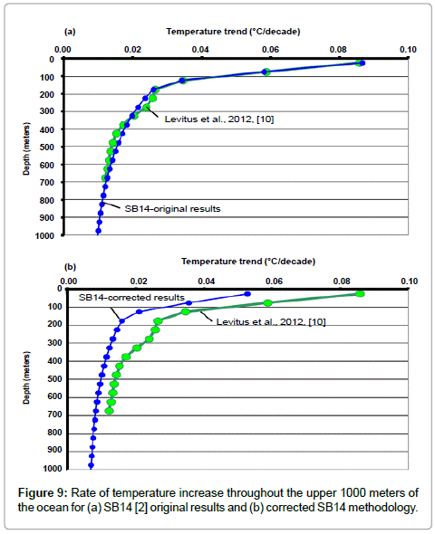
Figure 9: Rate of temperature increase throughout the upper 1000 meters of the ocean for (a) SB14 [2] original results and (b) corrected SB14 methodology.

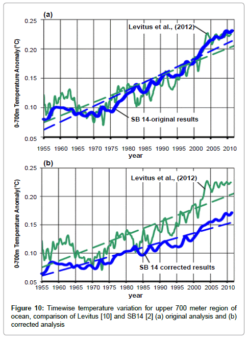
In oceanography research, changes to thermal energy in the upper 700 meters are typically classified as upper ocean heat content (0700OHC). The upper 700 meters is considered to be the most active zone of ocean in terms of energy storage. In fact, the 0-700 meter region absorbs approximately 50% of the extra heat added to the Earth climate system from increasing greenhouse gas concentrations.

Since it is seen that corrections to the simple one-dimensional diffusion model extend deep into the ocean, it remains to determine the impact of the SB14 errors on 0700OHC. Such a determination has been made in Figure 10. As before, the figure has two parts. The (a) part shows the original results from SB14 compared with the measurements of [10]. The (b) part of the figure shows the corrected results for the SB14 method alongside [10]. It is seen that the original results are in excellent agreement with the measurements, however, when the correct numerical methodology is employed, there is a significant difference in the evolution of ocean heating.

Figure 10: Timewise temperature variation for upper 700 meter region of ocean, comparison of Levitus [10] and SB14 [2] (a) original analysis and (b) corrected analysis

The results set forth in Figure 10, when considered alongside Figures 8 and 9 reveal significant deficiencies in the simplified model of SB14. It is generally accepted that simple climate models are a valuable tool to investigate the Earth’s climate system, however as clearly evident here; caution must be used to ensure that the proper numerical methodology is employed.

In each of the corrections, the SB14 results, when corrected, are found to significantly under-predict the temperatures and ocean heat content obtained from measurement.

A wide range of numerical models can be employed to study the Earth’s climate system. The models range from simple zero-dimensional calculations to complex three-dimensional simulations of both the atmosphere and oceans at a multitude of grid points deployed across the globe.

The focus of the present study is to evaluate the efficacy of simple one-dimensional ocean diffusion models which have been employed recently to suggest the Earth is not very sensitive to increasing carbon dioxide and other greenhouse gases. If true, this outcome would overturn decades of climate research and invalidate many state-of-theart climate models.

As shown here however, simple models can provide misleading and erroneous guidance when their core formulation is flawed. Through the use of a particular one-dimensional model as a case study, a number of shortcomings were identified in the formulation that invalidates their conclusions. Among the errors identified here are:

1. The model treats the entire Earth as ocean-covered

2. The model assigns an ocean process (El Nino cycle) which covers a limited geographic region in the Pacific Ocean as a global phenomenon (although the impacts of El Nino have global atmospheric implications).

3. The model incorrectly simulates the upper layer of the ocean in the numerical calculation.

4. The model incorrectly insulates the ocean bottom at 2000 meters depth

5. The model leads to diffusivity values that are significantly larger than those reported in the literature.

6. The model incorrectly uses an asymmetric diffusivity to calculate heat transfer between adjacent layers

7. The model contains incorrect determination of element interface diffusivity

8. The model neglects advection (water flow) on heat transfer

9. The model neglects latent heat transfer between the atmosphere and the ocean surface.

In the present study, focus was turned to the numerical algorithm, items 3, 4, 6 and 7. These corrections are applied to the original SB14 model and the impact of the corrections is shown. First, it is found that the surface temperature trend decreases by approximately 39% so that the model results and the measurements are no longer in agreement. Next, it is shown that the errors in the model extend deep into the ocean waters; significant model errors persist over the entire 700 meter depth for which measurements are available. Finally, the integrated average of the upper-ocean temperature is found to depart significantly from observations when these corrections are taken into account.

Taken together, this study shows that errors in one-dimensional numerical models have a significant impact on their ability to both match ocean measurements and serve as a check on more complex global models. Consequently, the conclusions based on these flawed models must be viewed with extreme skepticism and cannot be used as a surrogate for more complex and physically realistic models. While one-dimensional diffusion models have some use in climate studies, they must first be thoroughly evaluated and be grounded on a physically sound methodology. The analysis of SB14 is based on a model that fails these basic tests.

References

- Abraham JP, Baringer M, Bindoff NL, Boyer T, Cheng LJ, et al. (2013) A review of global ocean temperature observations: Implications for ocean heat content estimates and climate change. RevGeophys 51: 450-483.
- Spencer RW, Braswell WD (2014) The role of ENSO in global ocean temperature changes during 1955-2011 simulated with a 1D climate model. Asia Pacific J AtmosSci 50: 229-237.
- Oeschger H, Siegenthaler U, Schotterer U, Gugelmann A (1975) A box diffusion model to study carbon dioxide exchange in nature. Tellus 27: 168-192.
- Siegenthaler U (1983) Uptake of excess CO2 by an outcrop-diffusion model of the ocean. J Geophys Res 88: 3599-3608.
- Hoffert MI, Callegari AJ, Hsieh CT (1980) The role of deep sea heat storage in the secular response to climatic forcing. J Geophys Res 85: 6667-6679.
- Watts RG (1985) Global climate variation due to fluctuations in the rate of deep water formation. J Geophys Res 90: 8067-8070.
- Harvey LD, Schneider SH (1985) Transient climate response to external forcing on 10-10000 year time scales Part 1: Experiments with globally averaged, coupled, atmosphere and ocean energy balance models. JGeophys Res 90: 2191-2205.
- Harvey LD, Huang Z (2001) A quasi-one-dimensional coupled climate-change cycle model 1. Description and behavior of the climate component. J Geophys Res 106: 22339-22353.
- Harvey LD (2001) A quasi-one-dimensional coupled climate-change cycle model 2. The carbon cycle component. J Geophys Res 106: 22355-22372.
- Levitus S, Antonov JI, Boyer TP, Baranova OK, Garcia HE, et al. (2012) World ocean heat content and thermosteric sea level change (0-2000m), 1955-2010. Geophys ResLett 39: L10603.
- Patankar S (1980) Numerical Heat Transfer and Fluid Flow. Hemisphere Publishing Corporation, Washington, New York.
- Large WG, McWilliams JC, Doney SC (1994) Oceanic vertical mixing: A review and a model with a nonlocal boundary layer parameterization. Rev Geophys 32: 363-403.
Citation: Abraham JP, Kumar S, Bickmore BR, Fasullo JT (2014) Issues Related to the Use of One-dimensional Ocean-diffusion Models for Determining Climate Sensitivity. J Earth Sci Clim Change 5: 220. Doi: 10.4172/2157-7617.1000220
Copyright: ©2014 Abraham JP, et al. This is an open-access article distributed under the terms of the Creative Commons Attribution License, which permits unrestricted use, distribution, and reproduction in any medium, provided the original author and source are credited.
Share This Article
Open Access Journals
Article Tools
Article Usage
- Total views: 14329
- [From(publication date): 10-2014 - Apr 26, 2024]
- Breakdown by view type
- HTML page views: 9947
- PDF downloads: 4382