Long Term Trends in Mean Annual Surface, Mean Annual Maximum and Mean Annual Minimum Air Temperatures for Kolkata during 1941-2010
Received: 25-Feb-2014 / Accepted Date: 09-Apr-2014 / Published Date: 11-Apr-2014 DOI: 10.4172/2157-7617.1000197
Abstract
This study examines the changes in annual mean (minimum and maximum) temperatures for Kolkata weather observatory during 1941-2010. The analysis focus on the air temperature time series records at Alipore station (Kolkata) of Indian Meteorological Department (IMD). Variation and trend in annual mean temperature, annual mean maximum temperature and annual mean minimum temperature time series were statistically examined using CUSUM chart and bootstrapping techniques to identify the abrupt change in the considered data set. The major change (level 1) in the annual mean temperature occurred around 2001 with a rise of 1.417 °C. The numbers of change points in annual mean maximum and annual mean minimum temperature time series are detected at different levels but not at the level 1. Over the period under consideration (1941-2010), 4 forward and backward abrupt changes (1961, 1963, 1971 and 1991) are noticed in annual mean maximum temperatures, while 6 changes (1961,1964,1967,1974,1985 and 2003) are associated with the annual mean minimum temperature data set.
Keywords: Change point; Bootstrapping; CUSUM; Temperature Time Series
Introduction
In the last two or three decades a lot of researches concerning the nature of climatic fluctuations and trends of surface air temperature in different regions of the Earth have been carried out at various time scales. This type of research induced numerous trend detection studies on air temperature time series to test and confirm climate change concern. A study using reconstructed average of Land Surface Air Temperature (LST) data set by Smith [1] indicated an overall global scale warming throughout the Twentieth Century associated with a rise in mean surface temperature of about 0.6°C with an uncertainty estimate for the warming of ± 0.3°C. The study also indicates that there was a gradual land surface warming until about 1940 followed by a cooling between 1940 and 1970 and a second phase of warming trend began by about 1970. The successive periods of global warming, cooling and warming in the 20th century show distinctive patterns of temperature change suggestive of roles for both climate forcing and dynamical variables [2]. Many studies demonstrated that the observed warming trend during the past Century occurred mainly due to the growth in the average seasonal minimum temperatures rather than the average seasonal maximum temperatures. The increment in the minimum temperatures appeared mainly in the USA, former USSR, China and Australia [3,4]. This has been linked to several factors such as global warming, increased concentrations of anthropogenic greenhouse gases, aerosols (which also exerted cooling effects on the climate in many cases), increased cloud cover and urbanization [5,6]. The air temperature time series for the Northern Hemisphere seems to have the same rate of change, IPCC, 2001 [7]. In the South Asian region, the variations of the air temperature for the last few decades appear to be similar to the variations of temperature that have been recorded globally. According to the IPCC [7], the average global surface temperature increased by 0.74°C over the last 100 years [8]. One of the most significant potential consequences of climate change may be alterations in regional hydrological cycles [9]. General consensus has revealed that planetary warming and related alterations to the hydrological cycle are likely to raise the frequency and severity of extreme climate events, causing more serious floods and droughts [10-16].
Thus, the potential influence and relative importance of climate modification and human-induced perspectives of the change are the dominant factors that affect climatic parameters at the regional scale as well. In this concern, several studies showed that the variations of hydrological parameters such as precipitation, runoff, stream-flow, etc. are much more strongly related to regional climatic change. The key sources of error in the detection of abrupt changes in climatic data usually consist of the location of the observatory, changes of instruments, change in observation times, missing data and methods used to calculate daily or monthly means and increase of the urbanized area. So, it is difficult to establish the climatic trend, when in homogeneities of temperature time series occur as it may lead to misinterpretation of the results of investigation about climate change over any region. Hence, there is an earnest need for detecting change points in air temperature time series and adjustment of dataset thereby.
Study Area
Kolkata (22° C35' N and 88°30'E) the largest agglomeration as well as the capital city of the nation of India, West Bengal. Annual mean temperature is 26.8°C (80.2°F); monthly mean temperature ranges between 19°C to 30°C (66°F to 86°F). Summers (March-June) are hot and moderately humid, with temperature of 30°C in the low. During dry spells, maximum temperatures often exceed 40° C (104°F) in the month of May and June. Winter spell is very short; it lasts for only about two months, with a seasonal low temperature range between 9° C and 11°C (48°F to 52°F) in the month of December and January. May is the hottest month, with daily temperature ranging from 27°C to 37°C (81°F to 99°F); January, the coldest month, has temperatures varying from 12°C to 23°C (54°F to 73°F) as per the recent past climatological records. The highest recorded temperature is 43.9°C (111.0°F), and the lowest is 5°C (41°F), as measured at the Alipore weather observation station. During April-June, the city eventually experiences heavy rains or dusty squalls followed by thunderstorms or hailstorms, bringing cooling relief from the consisting high temperature and humidity in this region.
Data Base and Methods
The data used in this study were collected from the Eastern Regional Centre of Indian Meteorological Department, Kolkata (Alipore). The data consists of time series of year wise monthly average of maximum and minimum surface air temperature for the period ranging from 1941 to 2010 for the Kolkata weather observatory. Annual mean temperature for every year was calculated from the collected data and then it was statistically processed for further analysis. Studies of long-term climate change require that data be homogenous. Observed abrupt changes in a homogenous climate time series are caused only by variations in weather and climate [17]. In recent times several scientific studies have been conducted on quality control and homogenization of climatological data for the detection of climate trends [18-21]. Detailed explanations of the methods adopted for data analysis are as follows.
Cumulative Sum Charts (CUSUM) and Bootstrapping
The cumulative sum charts (CUSUM) and bootstrapping were performed as suggested by Taylor [22]. Let x1, x2,.... xn represents n data points of a time series, and Σ0 ,Σ1,Σ2 ,.....Σn are iteratively computed as follows
• The average of
 (1)
(1)
Let, Σ0 be equal to zero
Σi are computed recursively as follows
 (2)
(2)
i=1,2,....n
Actually, the cumulative sums are not the cumulative sums of the values. Instead, they are the cumulative sums of differences between the values and the average. These differences sum to zero, so the cumulative sum always ends at zero, Σn=0.
The confidence level can be determined for the apparent change by performing a bootstrap analysis [23,24]. Before performing the bootstrap analysis, an estimator of the magnitude of the change is required. One choice, which works well regardless of the distribution and despite multiple change is, Δi which is defined as
 (3)
(3)
Once the estimator of the magnitude of the change has been selected, the bootstrap analysis can be performed. A single bootstrap is performed by:
Generating a bootstrap sample of n data points of time series, denoted as xj (j=1,2,3…..n) by randomly reordering the original values. This is called Sampling Without Replacement (SWOR).
(b) Based on the bootstrap sample, the bootstrap CUSUM is calculated following the same method and denoted as, Σj
(c) The maximum, minimum and difference of the bootstrap CUSUM are calculated and the difference between the maximum and minimum bootstrap CUSUM is defined as,
 (4)
(4)
(d) Determine whether,
The bootstrap analysis consists of performing a large number of bootstraps and counting the number of bootstraps for which bootstraps difference Δj less than the original difference Δi. Let N is the number of bootstrap samples performed and let k be the number of bootstraps for which Δi < Δj . Then the confidence level that a change occurred as a percentage is calculated as follows:
Confidence Level
 (5)
(5)
Bootstrapping results in a distribution free approach with only a single assumption, that of an independent error structure.
Once a change has been detected, an estimate of when the change occurred can be made. One such estimator is the CUSUM estimator. Let i = m, such that:
 (6)
(6)
Then m is the point furthest from zero in the CUSUM chart. The point, m estimates last point before the change occurred. The point m+1 estimate the first point after the change. The second estimator of when the change occurred is the mean square error (MSE) estimator. Let MSE (m) be defined as:
 (7)
(7)
Where,
In MSE error estimation, the data series is split into two segments, 1 to m, and m+1 to n, then, it is estimated that how well the data in each segment fits their corresponding averages. The value of m, for which MSE (m) is minimized, gives the best estimate of the last point before change, while the point m+1 denote the first point after the change. In the same way, data of each segment can be passed through the above method to find level 2 change points that divide corresponding segments into sub-segments. Repetition of the procedure mentioned above helps finding significant change points at subsequent levels for each of which associated confidence limits and levels can be determined by bootstrapping. In this manner multiple change points can be detected by incorporating additional change points each at successive passes that will continue to split the segments into two. Once the change points, along with associated confidence levels, have been detected a backward elimination procedure is then used to eliminate those points that no longer qualify test of significance. To reduce the rate of false detection, when a point is eliminated, the surrounding change points are re-estimated along with their significance level. Thus the significant change points have been detected for the temperature time series considered for this study.
Variations and trends of annual mean temperature, annual mean minimum temperature and annual minimum temperature time series were examined following the method mentioned above. The Cumulative Sum Charts (CUSUM) and bootstrapping were used for the detection of abrupt changes. A section of the CUSUM chart with an ascending trend indicates a period when the values remaining above the overall average. Likewise, a section with a descending trend indicates a period of time where the values lie below the overall average. The confidence level can be determined by performing bootstrap analysis.
Results And Discussion
Fluctuations and change points detected in long term air temperature time series of annual mean maximum, annual mean minimum for Kolkata observatory are presented in Figure 1. The period of change has been indicated with a shaded background and maximum range of temperature fluctuation indicated by red lines under the situation of no change in trend. Table 1 describes confidence level and interval of these remarkable changes along with respective mean values of annual, annual maximum and annual minimum temperature. The table indicates a level associated with each of the changes signifying the importance of the change. The level 1 change indicates the first change which is most visibly apparent in the CUSUM chart. The level 2 changes have been detected on passing the data through the analytical process for the second time. Thus, every change point is associated with a particular importance level. There are four change points, including level 1 change in annual mean average temperature dataset (Table 1a), four changes in annual mean maximum temperature without any level 1 change (Table 1b) and six points of change none of which is a level 1 change.
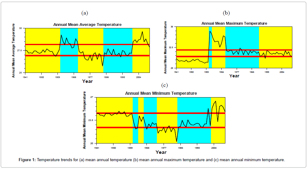
Figure 1: Temperature trends for (a) mean annual temperature (b) mean annual maximum temperature and (c) mean annual minimum temperature.
| (a): Table for Significant Changes for Annual Mean Average Temperature. | |||||
| Year | Confidence Interval | Conf. Level | From | To | Level |
| 1961 | (1961, 1962) | 100% | 27.35 | 28.445 | 5 |
| 1971 | (1971, 1971) | 100% | 28.445 | 26.833 | 3 |
| 1985 | (1972, 1990) | 98% | 26.833 | 27.209 | 2 |
| 2001 | (2001, 2002) | 100% | 27.209 | 28.626 | 1 |
| (b): Table for Significant Changes for Annual Mean Maximum Temperature | |||||
| Year | Confidence Interval | Conf. Level | From | To | Level |
| 1961 | (1961, 1962) | 94% | 30.232 | 35.082 | 4 |
| 1963 | (1963, 1966) | 97% | 35.082 | 33.64 | 3 |
| 1971 | (1970, 1971) | 100% | 33.64 | 31.767 | 2 |
| 1991 | (1983, 2002) | 94% | 31.767 | 31.421 | 4 |
| (c): Table for Significant Changes for Annual Mean Minimum Temperature | |||||
| Year | Confidence Interval | Conf.Level | From | To | Level |
| 1961 | (1961, 1961) | 98% | 24.445 | 22.539 | 2 |
| 1964 | (1963, 1964) | 97% | 22.539 | 23.871 | 5 |
| 1967 | (1966, 1967) | 90% | 23.871 | 22.834 | 4 |
| 1974 | (1973, 1984) | 95% | 22.834 | 21.902 | 6 |
| 1985 | (1982, 1986) | 100% | 21.902 | 23.004 | 5 |
| 2003 | (2002, 2004) | 100% | 23.004 | 25.352 | 3 |
Table 1: Significant change in (a) mean annual average temperature series, (b) mean annual maximum temperature series and (c) mean annual minimum temperature series.
Using the Change Point Analyzer, no departure from the independent error structure and no outlier’s assumption were found. The errors are positively correlated, which means that if the single value is above average temperature trend, the next several values will also tend to be above average. Though the results of the analysis may incorrectly indicate that a change has taken place, but the associated level of confidence adaptive from bootstrapping may confirm the change to have occurred. This analysis indicates that the annual mean temperature reveals a quasi-change in the year of 1961 and 1971 (Confidence intervals 1961-1962 and 1971) respectively. Both of them have occurred at the 100% confidence level, at level-5 and level-3 respectively. This analysis, using CUSUM and the bootstrapping method reveals that the largest change in mean annual temperature by a magnitude of 1.417°C in associated with 2001 within the interval period of one year in temporal scale. Prior to the change in 2001 at level 1, annual mean temperature was 27.209°C, while subsequent to the change the average temperature became 28.626°C. In accordance to this analysis, it has been noted that a level 2 abrupt change in mean annual temperature took place in the year 1985 (Confidence interval 1972-1990), at a confidence level of 98%. Prior to change in 1985, the annual mean temperature was 26.833°C; while after the change of mean annual temperature became 27.209°C.
Analysis of the mean maximum time series shows that the average value changed significantly from 30.232°C to 35.082°C by the year 1961 (Confidence level 94%; level 4), from 35.082°C to 33.64°C by 1963 (Confidence interval 1963, 1966; Confidence level 97%; level 3), from 33.64°C to 30.767°C by 1971 (Confidence interval 1970, 1971; Confidence and 100%; level 2) and from 31.767°C to 31.421°C by 1991 (Confidence interval 1983, 2002; Confidence level 94%; level 4). The amount of change of mean annual maximum temperature time series associated with the change points were 4.85°C, 1.38°C, 1.87°C and 0.346°C, respectively (Table 1b). On the other hand, the mean minimum temperature time series indicates six significant changes. Among them, the changes in 1985 and 2003 are identified at the 100% confidence level with confidence intervals 1982 to 1986 and 2002 to 2004, respectively. Prior to the six changes in 1961,1964,1967,1974,1985 and 2003, the annual mean minimum temperature were 24.445°C, 22.539°C, 23.871°C, 22.834°C, 21.902°C and 23.004°C respectively, while after these changes, the annual mean minimum temperature changed to 22.539°C, 23.871°C, 22.834°C, 21.902°C, 23.004°C and 25.352°C, respectively (Table 1c). Over the entire period considered (1941-2010), 14 forward and backward changes were found.
In general it can be said that most of the tendencies in this analysis showed increase in trend in temperatures time series. The effect of urbanization is usually reflected in the increase in mean minimum temperature. Besides this, station location, instrumentation and change in surrounding environment may have been amplified the same in the regards of said change. The inhomogeneity is an unadjusted temperature time series is often attributed to change in instrumental arrangements and/or measuring conditions. But if such was the case in present context, all the data sets would have supposedly indicated changes within approximation of common range of years which could not be found in case of Kolkata. Hence, the change in temperature trend may be due to rapid urbanized area, expansion of industrial activities, and these areas are a sort of heat island since 1980s. From these analysis results it can be inferred that though urbanization and industrial activities is leading to changing the temperature time series in the station, it is not the case always. Secondly, the rate of change in temperature, in rapidly urbanized area may vary. The urbanization and industrial activities was also dealt with by adopting a different approach in which combined effect of the population and temperature change in this study has been considered for the explanation.
The CUSUM charts are presented in Figure 2. The analysis is important to identify the single or multiple change points over the period under study. The annual mean temperature CUSUM chart (Figure 2a) exhibits abrupt changes at most four times which occurred in 1961, 1971, 1985 and 2001. The first and most important change point is estimated to have occurred around 2001 with 100% confidence level. Prior to 2001 average annual mean temperature was found to be 27.2°C while after the first change it was 28.6°C (Table 1a).
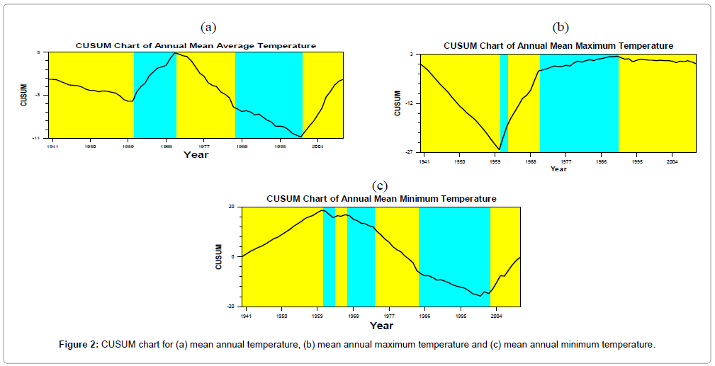
Figure 2: CUSUM chart for (a) mean annual temperature, (b) mean annual maximum temperature and (c) mean annual minimum temperature.
After these level 5 changes, the annual average temperature chart line goes upward till 1971 and then the chart line gradually goes downward till 2001 Figure 3. Within this period of decreasing trend from 1971-2001, a level 2 change points have been detected in 1985 at 98% confidence level with a confidence interval of 18 years in temporal scale. Forth more, the plots of CUSUM line goes gradually upward till 2010. In case of the annual mean minimum temperature, the decreasing trend period is less than the span of increasing trend over the entire period; these intervals are 20 years & 49 years, respectively. In the first ten years (1961-1971) increase was rapid and after forty-nine years (1972-2010) annual average maximum temperature exhibits an almost stabling. From first to last sequential change points, the average amount of change is 1.19°C. On the other hand, analysis with the annual mean minimum temperature has led to finding at most six change points over the period. According to the CUSUM chart, the rising trend is detected till 1961 and after that, the plots of CUSUM values have indicated a decreasing trend till 2003. Then it further goes upward rapidly, indicating a rising trend till 2010. The value of the average of annual mean minimum temperature for this period is above the overall average of annual mean temperature (25.35°C). Figure 4 presents that there is no significant change in annual mean and annual mean maximum or annual mean minimum temperatures standard deviations.
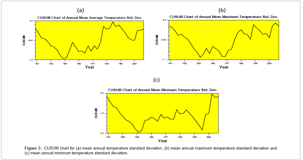
Figure 3: CUSUM chart for (a) mean annual temperature standard deviation, (b) mean annual maximum temperature standard deviation and (c) mean annual minimum temperature standard deviation.
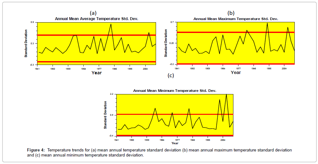
Figure 4: Temperature trends for (a) mean annual temperature standard deviation (b) mean annual maximum temperature standard deviation and (c) mean annual minimum temperature standard deviation.
Conclusion
Above results may look as if simple to interpret but are in fact so very complex. In this analysis, the 70 years long term air temperature time series of annual mean, annual mean maximum and annual mean minimum temperature has been compiled and statistically analyzed. The CUSUM analysis has been performed to identify the change points in every series and bootstrapping has been performed to determine significance level associated with each of the detected change points. This analysis confirms a major change in annual mean temperature of Kolkata observatory to have occurred around 2001 at level 1. Application of CUSUM chart clearly demonstrates the annual mean, annual mean maximum and annual mean minimum temperature trends. The analysis of annual mean minimum temperatures showed a significant warming trend after the change point in 2003. In change point analysis, the results significantly depend upon the period of data and the stations whose data are used. There is a another observation that the data used in change point detection pertaining to the said station in that are located rapid urbanized area, expansion of industrial activities, and these areas are a sort of heat island since 1980s. Thus, the analysis of change points using this data may not be the correct depiction of the reality and this aspect need to be addressed. Change in annual mean minimum temperatures due to urbanization effect. However, Changes at Kolkata pose a question. Secondly, if the effect of urbanization is dominant, mean minimum temperatures should have increased at higher rates than mean maximum. On the other hand, effect of urbanization is not similar in all seasons. One important aspect of Indian climate is its dominance by south west monsoon onset and circulation. This in turn is controlled by many other global and regional factors. Analysis of these factors was outside the scope of this research. It is quite possible that the changes in lower atmosphere may be responsible for variations and detections observed at Kolkata weather observatory. Thus, it is worthwhile emphasizing that the results of the present study are not sufficient to approve change point in temperature time series and subsequent climate change at Kolkata weather observatory. Future studies with longer data recorded and several stations are essential to check change point in temperature time series and its attributes in Kolkata, especially in sub-tropical regions of India.
References
- Smith TM, Reynolds WR (2005) A global merged land-air-sea surface temperature reconstruction based on historical observations. J Climate 18: 2021-2036.
- Hansen JE, Ruedy R, Sato M, Imhoff M, Lawrence W, et al.(2001) A closer look at United States and global surface temperature change. J Geophys Res 106: 23947-23963.
- Folland CK, Karl TR, Nicholls N, Nyenzi BS, Parker DE,et al.(1992) Observed climate variability and change', Climate Change. The Supplementary Report to the Intergovernmental Panel on Climate Change Scientific Assessment, Cambridge University Press, UK.
- Karl TR, Kukla G, Razuvayev VN, Changery MJ, Quayle RJ, et al.(1991) Global warming evidence for asymmetric diurnal temperature change. Geophys Res Lett 18: 2253-2256.
- Balling RC(1992) The heated debate: Greenhouse predictions versus climate reality. Pacific Research Institute for Public Policy, San Francisco, USA.
- Englehart PJ, Douglas AD(2003) Urbanization and seasonal temperature trends: Observational evidence from a data-sparse part of North America. Intl J Climatol 23: 1253-1263.
- IPCC (2001) Third Assessment Report, Working Group-I Report. Cambridge University Press, Cambridge, UK.
- IPCC (2007) Climate change 2007: the physical science basis. Contribution of Working Group I to the Fourth Assessment Report of the Intergovernmental Panel on Climate Change. Cambridge University Press, Cambridge, UK.
- Huntington TG (2006) Evidence for intensification of the global water cycle: review and synthesis. J Hydrol 319: 83-95.
- Milliman JD, Farnsworth KL, Jones PD, Xu KH, Smith LC(2008) Climatic and anthropogenic factors affecting river discharge to the global ocean, 1951–2000. Global Planet Change 62: 187-194.
- Bates BC, Kundzewicz ZW, Wu S, Palutikof JP(2008) Climate Change and Water. Technical Paper of the Intergovernmental Panel on Climate Change. IPCC Secretariat, Geneva.
- Déry SJ, Hernández-Henríquez MA, Burford JE, Wood EF(2009) Observational evidence of an intensifying hydrological cycle in northern Canada. Geophys Res Lett 36: L13402.
- Jung G, Wagner S, Kunstmann H(2012) Joint climate-hydrology modeling: an impact study for the data-sparse environment of the Volta Basin in West Africa. Hydrol Res 43: 231-248.
- Thompson JR(2012) Modelling the impacts of climate change on upland catchments in southwest Scotland using MIKE SHE and the UKCP09 probabilistic projections. Hydrol Res 43: 507-530.
- Li L, Ngongondo CS, Xu CY, Gong L (2012) Comparison of the global TRMM and WFD precipitation datasets in driving a large-scale hydrological model in Southern Africa. Hydrol Res 44: 5.
- Xiong LH, Yu KX, Zhang HG, Zhang LP(2013) Annual runoff change in the headstream of Yangtze River and its relation to precipitation and air temperature. Hydrol Res 44: 850.
- Serra C, Burgueno A, Lana X (2001) Analysis of maximum and minimum daily temperatures recorded at fabra observatory (Barcelona, NE Spain) in the period 1917–1998. Int J Climatol 21: 617-636.
- Peterson TC, Easterling DR, Karl TR (1998) Homogeneity Adjustments of in Situ Atmospheric Climate Data: A Review. Int J Climatolol 18: 1493-1517.
- Karl TR, Williams CN Jr (1987) An Approach to Adjusting Climatological Time Series for Discontinuous In-TACT>2.0.C homogeneities. J ClimAppl Meteorol26: 1744-1763.
- Alexanderson H (1986) A Homogeneity Test Applied to Precipitation Data. J Climatol 6: 661-675.
- Buishan TA (1982) Some Methods for Testing the Homogeneity of Rainfall Records. J Hydrol 58:11-27.
- Taylor W (2000) Change-Point Analysis: A Powerful Tool for Detecting Changes. Taylor Enterprises, Libertyville, USA.
- Taylor W (2000) Change-Point Analyzer 2.3 Software Pack- age. Taylor Enterprises, Libertyville, USA.
- Davison AC, Hinkley DV (1997) Bootstrap Methods and Their Application. Cambridge University Press, Cambridge, UK.
Citation: Bisai D, Chatterjee S, Khan A (2014) Long Term Trends in Mean Annual Surface, Mean Annual Maximum and Mean Annual Minimum Air Temperatures for Kolkata during 1941-2010. J Earth Sci Clim Change 5: 197. Doi: 10.4172/2157-7617.1000197
Copyright: © 2014 Bisai D, et al. This is an open-access article distributed under the terms of the Creative Commons Attribution License, which permits unrestricted use, distribution, and reproduction in any medium, provided the original author and source are credited.
Share This Article
Open Access Journals
Article Tools
Article Usage
- Total views: 14458
- [From(publication date): 7-2014 - Apr 27, 2024]
- Breakdown by view type
- HTML page views: 10062
- PDF downloads: 4396