A Decision Support Tool for Selection of Suitable General Circulation Model and Future Climate Assessment
Received: 03-Aug-2012 / Accepted Date: 26-Sep-2012 / Published Date: 28-Sep-2012 DOI: 10.4172/2157-7617.1000117
Abstract
It is widely accepted that General Circulation Models (GCMs) are physically based means for formulating climate scenarios. At the global and continental scale the climate prediction is good but GCMs may not provide the required climate features, in many of the regional and local-scale processes, which are needed for climate change impact studies. Therefore, downscaling is required to develop climate scenarios of higher spatial resolutions. Also the simulated data for different GCMs is freely available at IPCC data distribution Centre, but to extract the data for a particular region and convert it to a user readable format, different software packages are required. This study presents a decision support tool to select a suitable GCM for any specific region, based on statistical parameters such as coefficient of determination (R2) and Root Mean Square Error (RMSE). The tool also provides the facility to obtain the simulated data for different GCMs in the excel format. Delta change method is incorporated as a downscaling technique to project future climate scenarios. To demonstrate the application of the tool, future air surface temperature and precipitation scenarios are projected for 2021-2050, using data for four meteorological stations from upper Jhelum basin, Pakistan.
Keywords: Climate change; Delta change; GCM; Downscaling
8657Introduction
The rising concentration of greenhouse gases in the atmosphere due to human activities such as land use changes and dependence upon fossil fuels has led to global warming and global energy unbalance [1-4]. Fourth Assessment Report (4AR) of the Intergovernmental Panel on Climate Change (IPCC) had reported a 0.74°C increase in the global mean surface temperature during the last hundred years (1906- 2005). In the last 50 years a significant increase has been reported with an increasing rate of 0.13°C every 10 years. The global mean surface temperature is projected to increase approximately from 1.1 to 6.4°C during the 21st century [5]. This increased global warming can affect the hydrological cycle, water resources, public health, industrial and municipal water demands, water energy exploitation and the ecosystem [2,6]. It is widely consented that General Circulation Models (GCMs) are physically based means for formulating climate scenarios [7]. At the global and continental scale the climate prediction is good [8], but GCMs may not provide the required climate features in many of the regional- and local-scale processes that are needed for climate change impact studies [9,10]. This is due to the coarse spatial resolution of GCMs which limits their effectiveness at smaller scales [9]. Another reason for this gap is the inadequate parameterization of various processes (e.g., evapo-transpiration, soil moisture) concerning cloud formation and land surface interactions with the atmosphere [7]. Therefore, some type of downscaling, such as statistical downscaling, dynamic downscaling, or the delta change method is required to develop scenarios of higher temporal and/or spatial resolutions than presently produced by GCMs [10]. However each of these downscaling techniques has its advantages and limitations.
Dynamic downscaling embeds Regional Climate Models (RCMs) within large-scale GCMs. RCMs interpret atmospheric processes running at small scales for GCMs, such as orographic rainfall and surface–atmosphere interactions [11,12]. However, RCMs involve a huge number of thermodynamics equations and therefore RCMs are computationally expensive and complex [10,12].
Statistical downscaling presumes that large-scale atmospheric processes and regional forces affect regional climates [12-14]. To predict regional-scale climate changes the statistical relationships between large scale climate variables and local variable, are found out from observed data and then applied to the GCM simulations [12]. Since the relationships between local and large-scale variables differ as a function of a land-space, therefore most of the statistical downscaling studies are restricted to individual regions [15,16]. Another problem with this technique is that it presumes that the relationships between large-scale climate variables and local variables always remain the same [12].
There are many studies where the inter-comparison of different downscaling techniques has been made (e.g. [17-20]). The fastest technique used for global-scale downscaling of a large number of climate simulations is the change factor method [12,13,21-23], often named as “delta change”. This approach has been widely used in climate change research e.g., reproducing future climate scenarios for high-resolution modeling of flora and bionomical sensitivity to climate change in United States [12].
As described above GCM data is widely used for the analysis of climate change impacts on agriculture and biodiversity. For different GCMs the data is freely available [24], but in many cases the data cannot be used in its existing format for further processing. Software tools (e.g. Climate Date Operators (CDO), PANOPLY) are required to convert that data into ASCII or Excel format [25]. In this study a tool is developed to provide the user with the facility to obtain the data for different GCMs in Excel format, by using the corresponding latitude and longitude as input. After obtaining the GCM simulated data, the user can compare the observed data with the GCM output, and based on the statistical parameters can find out which GCM is most suitable for the corresponding region. Delta change method is incorporated as a downscaling method to obtain future climate scenarios for the given region.
Data and Sources
Using various GCMs the impacts of the IPCC emission scenarios on global/local climates have been determined. To present possible future changes SRES (Special Report on Emission Scenario) focuses on future concentrations and emissions of greenhouse gases and applies four main socio-economic future trends (A1, A2, B1 and B2). Here we have used the historical 20C3M scenario as well as the projected A1, A1B, A2, and B2 datasets for downscaling. For global solutions A1 and B1 scenarios are focused, while for regional solution A2 and B2 scenarios are used. Scenarios A1 and A2 forecast an increase in cumulative emissions between 1990-2100, whereas B1 and B2 predict that emissions will balance with time [26]. The details about various GCMs experiments under various scenarios are described in the IPCC (2001a-2007) report [5,27]. GCM simulated data for all models is available at the IPCC Data Distribution Center. Table 1 depicts summary of the models used in the study. The two important and commonly used parameters (i.e. temperature and precipitation) are evaluated.
| Modeling Centre | SRES Scenarios | Resolution | Country Developed |
| CCCma | A2 | 3.75°x3.75° | Canada |
| CCCma | B2 | 3.75°x3.75° | |
| CCCma | 20C3M | 3.75°x3.75° | |
| CCSRNIES | A2 | 5.6°x5.6° | Japan |
| CCSRNIES | A2 | 5.6°x5.6° | |
| CCSRNIES | 20C3M | 5.6°x5.6° | |
| CSIRO-Mk2 | A2 | 3.2°x5.6° | Australia |
| CSIRO-Mk2 | B2 | 3.2°x5.6° | |
| CSIRO-Mk3 | 20C3M | 1.8°x1.8° | |
| ECHAM | A2 | 2.8°x2.8° | Germany |
| ECHAM | B2 | 2.8°x2.8° | |
| ECHAM | 20C3M | 2.8°x2.8° | |
| HadCM3 | A2 | 2.5°x3.75° | UK |
| HadCM3 | B2 | 2.5°x3.75° | |
| HadCM3 | 20C3M | 2.5°x3.75° |
Table 1: Characteristics of different GCMs.
GCM evaluation and future climate projection
The main purpose of developing this software is to provide a user friendly tool for the researchers, to obtain suitable GCM simulated data for accessing climate impacts as well as to project future climate scenarios using delta change method.
GCM evaluation: As discussed above, to evaluate different GCMs, statistical parameters such as coefficient of determination (R2) and root mean square error (RMSE) are used.
• Coefficient of determination (R2): It is the square of correlation coefficient (R) and shows the proportion of the variance of variable Oi from variable Si.
 (1)
(1)
Where R is the correlation coefficient, n denotes number of months; Oi and Si represent observed and simulated monthly data respectively.
• Root mean square error (RMSE): It quantifies the patterns similarity by measuring the differences between values predicted by the model and the values actually observed.
 (2)
(2)
Where n denotes number of months, Oi and Si represent observed and simulated monthly data respectively.
Future climate projection: For future climate projection delta change approach is used, which has been employed before in many studies [21,23,28,29]. This method adapts observed climate time series with estimated monthly GCM simulated data.
The future daily precipitation (Pf, daily) and temperature (Tf, daily) are constructed as given in Eqs. (3) and (4) respectively
 (3)
(3)
 (4)
(4)
where Po,daily is the observed daily precipitation, Pf,monthly is the GCM predicted future mean monthly precipitation, Pp,monthly is the present mean monthly GCM simulated precipitation, where To,daily is the observed daily temperature, Tf,monthly is the GCM predicted future mean monthly temperature, Tp,monthly is the present mean monthly GCM simulated temperature.
Design and application of the tool
The software is developed under the Matlab environment [30]. The general frame work and software interface are shown in Figure 1 and Figure 2 respectively. The software shortens the task of; obtaining GCM data, evaluation of different GCMs, and future climate projection using “delta change” technique in three steps.
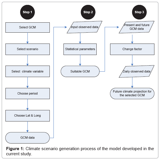
Figure 1: Climate scenario generation process of the model developed in the current study.
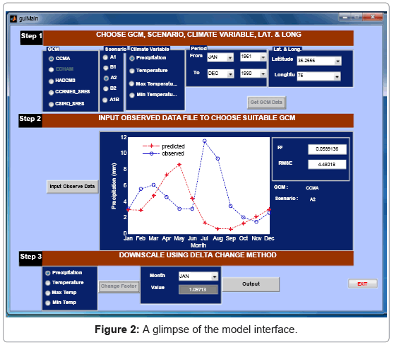
Figure 2: A glimpse of the model interface.
Obtain GCM data: Simulated data for different GCMs is freely available at the IPCC [31], data distribution Centre [32], but after downloading the data some software tools (e.g. CDO,PANOPLY) are needed to convert the data into user readable format. The purpose of ‘obtain GCM data’ operation is to assist the user to obtain the GCM simulated data for the corresponding latitude & longitude in excel format. To carry out the operation the user has to select the GCM model, scenario, climate variables (precipitation, temperature, maximum temperature, and minimum temperature), time period, and latitude & longitude.
Choose suitable GCM: Several climate models with different scenarios have projected the climate change in the globe for the 21st century. Some studies showed that the climate models have the certain capacities to simulate the climate change at the global and continental scale (IPCC 2001b) [32].
This software has focused on two climate variables, surface temperature (mean, maximum, minimum) and precipitation. ’Choose suitable GCM’ operation gives the facility to find out suitable GCM, based on its ability to simulate the present climate in a better way after comparison with the observed data [33]. Once the data has been entered, the software reports the user with information which includes statistical parameters such as coefficient of determination (R2) and Root Mean Square Error (RMSE) as shown in Figure 3. The R2 and RMSE values present complementary statistical information which shows the correspondence between two patterns. A low value of R2 is associated with a high RMSE and vice versa. The closeness of R2 and RMSE values indicate that a model is effective for simulating the magnitude of variance.
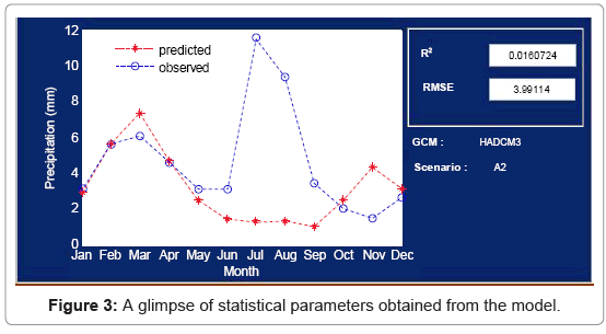
Figure 3: A glimpse of statistical parameters obtained from the model.
Future climate projection: Delta change method is being used for future climate scenarios projection. This method has been employed in many studies [21,23,28,29]. Once the two data sets of the same period for present and future GCM data are given, software reports the user with the value of change factor for each month. These values are then used to generate future climate scenarios for precipitation and temperature using Eqs. (3) and (4) respectively.
An illustration of the model application
Application of the tool is demonstrated with respect to future temperature and precipitation scenarios projection, for upper Jhelum basin, Pakistan. Table 2 lists some features of the meteorological stations and Figure 4 shows the location of the stations. The observed data set is obtained from Water and Power Development Authority (WAPDA) and Pakistan Meteorological Department (PMD), Pakistan. Mean monthly precipitation along with minimum and maximum temperature data at four stations in upper Jhelum basin, for the period 1961-1990 is used.
| Station | Latitude | Longitude | Period of record | Elevation (meters) |
| Balakot | 34°.55' | 73°.35' | 1961-1990 | 995.4 |
| Garhi dopatta | 34°.22' | 73°.62' | 1961-1990 | 813.5 |
| Muzaffar abad | 34°.37' | 73°.48' | 1961-1990 | 702 |
| Naran | 34°.90' | 73°.65' | 1961-1990 | 2362 |
Table 2: Meteorological stations used for analysis in upper Jhelum basin, Pakistan.
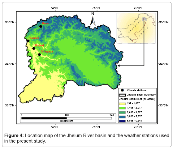
Figure 4: Location map of the Jhelum River basin and the weather stations used in the present study.
The process began with the selection of GCM, scenario, climate variable, time period, and latitude & longitude for the target site (Figure 4), which resulted in the production of GCM simulated data for the specified region. After the GCM simulated data for the period 1961-1990 was obtained, then the observed data for the same period was given as input to find out the suitable GCM for the specified region based on statistical parameters, namely, R2 and RMSE. Various GCMs simulations and observed data showed a significant variability as shown in Tables 3 and 4.
| Station | CCCma | HadCM3 | SRNIES | CSIRO | |||||
| A2 | B2 | A2 | B2 | A2 | B2 | A2 | B2 | ||
| Balakot | R2 | 0.92 | 0.92 | 0.97 | 0.97 | 0.94 | 0.94 | 0.96 | 0.96 |
| RMSE | 22.3 | 22.3 | 22.45 | 22.42 | 9.57 | 9.57 | 11.44 | 11.44 | |
| Garhi Dopatta | R2 | 0.94 | 0.94 | 0.98 | 0.98 | 0.95 | 0.95 | 0.97 | 0.97 |
| RMSE | 22.96 | 22.98 | 23.16 | 23.13 | 10.14 | 10.14 | 12.12 | 12.12 | |
| Muzaffar Abad | R2 | 0.93 | 0.93 | 0.97 | 0.97 | 0.95 | 0.95 | 0.96 | 0.96 |
| RMSE | 24.16 | 24.18 | 24.36 | 24.33 | 11.3 | 11.3 | 13.31 | 13.31 | |
| Naran | R2 | 0.97 | 0.97 | 0.96 | 0.96 | 0.96 | 0.96 | 0.94 | 0.94 |
| RMSE | 10.29 | 10.31 | 10.19 | 10.17 | 5.19 | 5.18 | 2.85 | 2.85 | |
Table 3: Comparison of statistical parameters obtained from different GCMs relative to observed temperature for the period 1961-1990 for the upper Jhelum basin.
| Station | CCCma | HadCM3 | SRNIES | CSIRO | |||||
| A2 | B2 | A2 | B2 | A2 | B2 | A2 | B2 | ||
| Balakot | R2 | 0.059 | 0.06 | 0.01 | 0.02 | 0.004 | 0.004 | 0.0 | 0.0 |
| RMSE | 4.48 | 4.5 | 4.0 | 4.0 | 4.73 | 4.73 | 4.9 | 4.9 | |
| Garhi Dopatta | R2 | 0.06 | 0.07 | 0.02 | 0.02 | 0.003 | 0.003 | 0.0 | 0.0 |
| RMSE | 3.80 | 3.82 | 3.27 | 3.28 | 3.97 | 3.97 | 4.12 | 4.12 | |
| Muzaffar Abad | R2 | 0.04 | 0.04 | 0.003 | 0.003 | 0.0 | 0.0 | 0.005 | 0.005 |
| RMSE | 3.59 | 3.60 | 3.0 | 3.0 | 3.53 | 3.53 | 3.70 | 3.70 | |
| Naran | R2 | 0.24 | 0.24 | 0.74 | 0.73 | 0.97 | 0.97 | 0.86 | 0.86 |
| RMSE | 2.18 | 2.19 | 0.96 | 0.97 | 2.35 | 2.36 | 2.47 | 2.47 | |
Table 4: Comparison of statistical parameters obtained from different GCMs relative to observed precipitation for the period 1961-1990 for the upper Jhelum basin.
The GCMs showed good results while simulating the spatial variability of mean temperature. Every model had responded with a high value of R2 (0.91-0.96), suggesting that they were accurate at representing the spatial pattern of variation. But all the models substantially underestimated the magnitude of monthly temperature for the period 1961-1990, as shown in Table 3. The possible reason for this underestimation is the hilly nature of the study area, , where the stations are located at low elevation as shown in Figure 4. The GCM simulated annual cycle of temperature had reported December or January as the coldest month and Jun or July as the warmest, which indicates that the annual cycle is qualitatively similar to the observations.
Every GCM model showed higher variations for precipitation than those for mean temperature. Unlike temperature cycle, GCM simulated annual cycle for precipitation was not able to produce observed annual cycle even qualitatively similar, as shown in Figure 5 and Figure 6. IPCC (2001b) report describes that no model can be considered as the best, therefore a couple of models should be used for climate change analysis. [32].
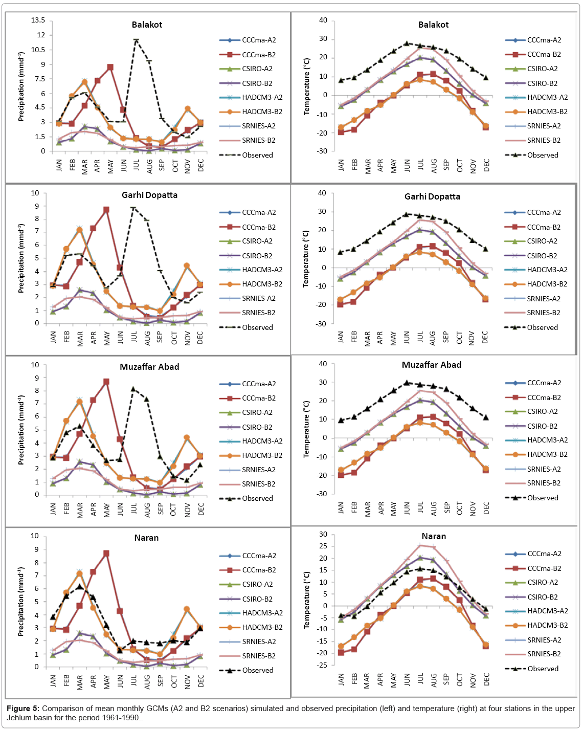
Figure 5: Comparison of mean monthly GCMs (A2 and B2 scenarios) simulated and observed precipitation (left) and temperature (right) at four stations in the upper Jehlum basin for the period 1961-1990.
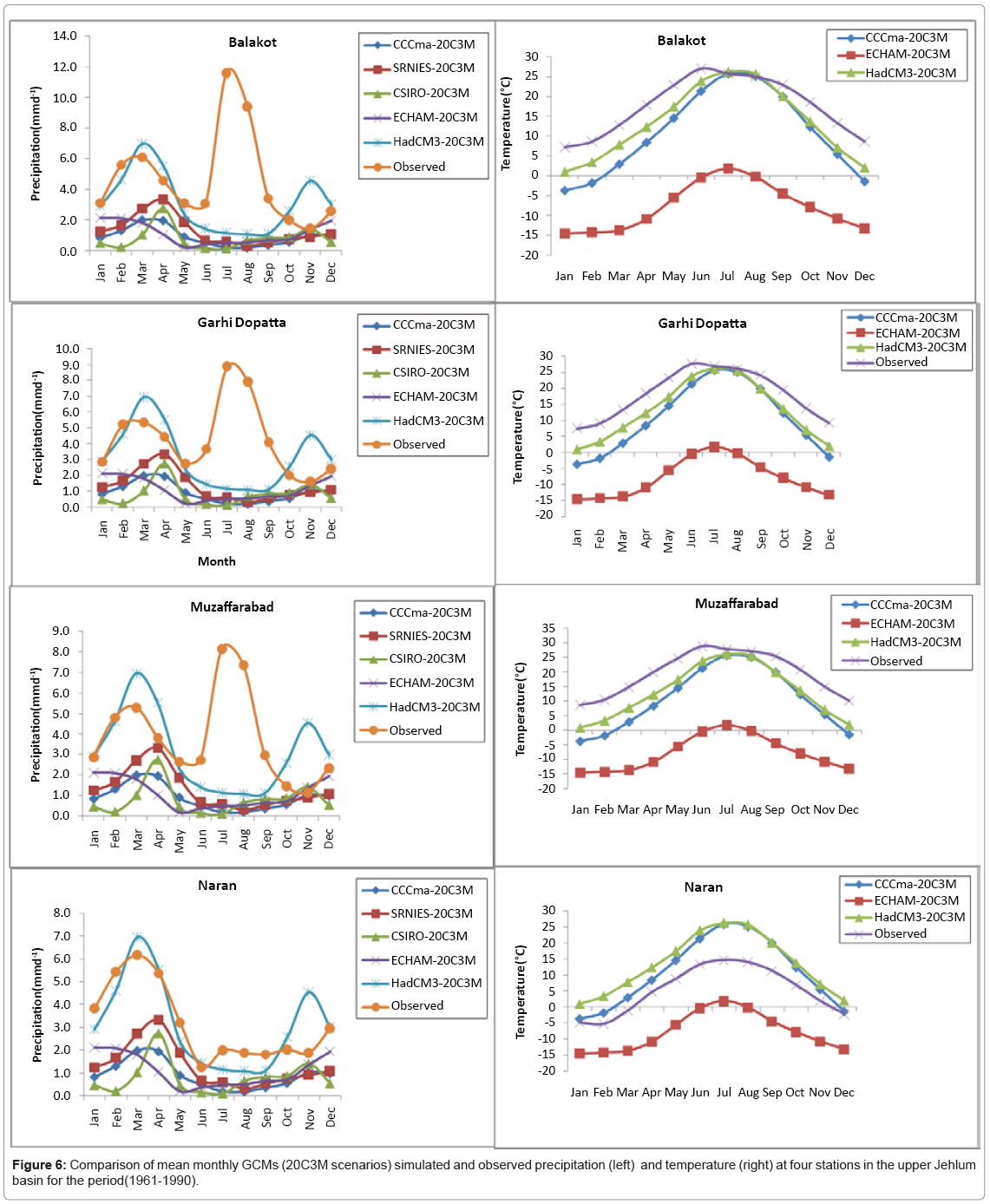
Figure 6: Comparison of mean monthly GCMs (20C3M scenarios) simulated and observed precipitation (left) and temperature (right) at four stations in the upper Jehlum basin for the period(1961-1990).
The validity of the model is assessed by projecting mean monthly temperature and precipitation for the past time period (1981-1990) relative to 1971-1980, and then analyzing the statistical relationship between observed and projected data for the same period. This analysis examined the degree to which the observed and projected mean monthly temperature and precipitation matches. For each of the four stations, scatter plots were created in which the projected temperature and precipitation for each month from 1981-1990 was graphed against the observed mean for that month as shown in Figure 7 and Figure 8. The model shows a close fit between projected and observed temperature with R2 values ranging from 0.94 to 0.98, where as R2 values are lower for precipitation ranging from 0.1 to 0.6.
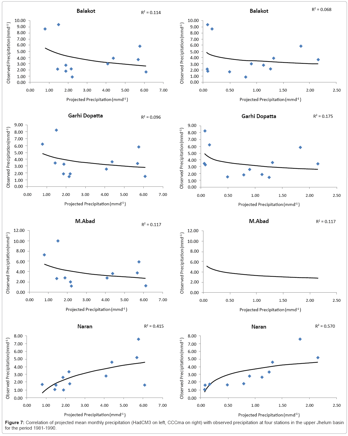
Figure 7: Correlation of projected mean monthly precipitation (HadCM3 on left, CCCma on right) with observed precipitation at four stations in the upper Jhelum basin for the period 1981-1990.
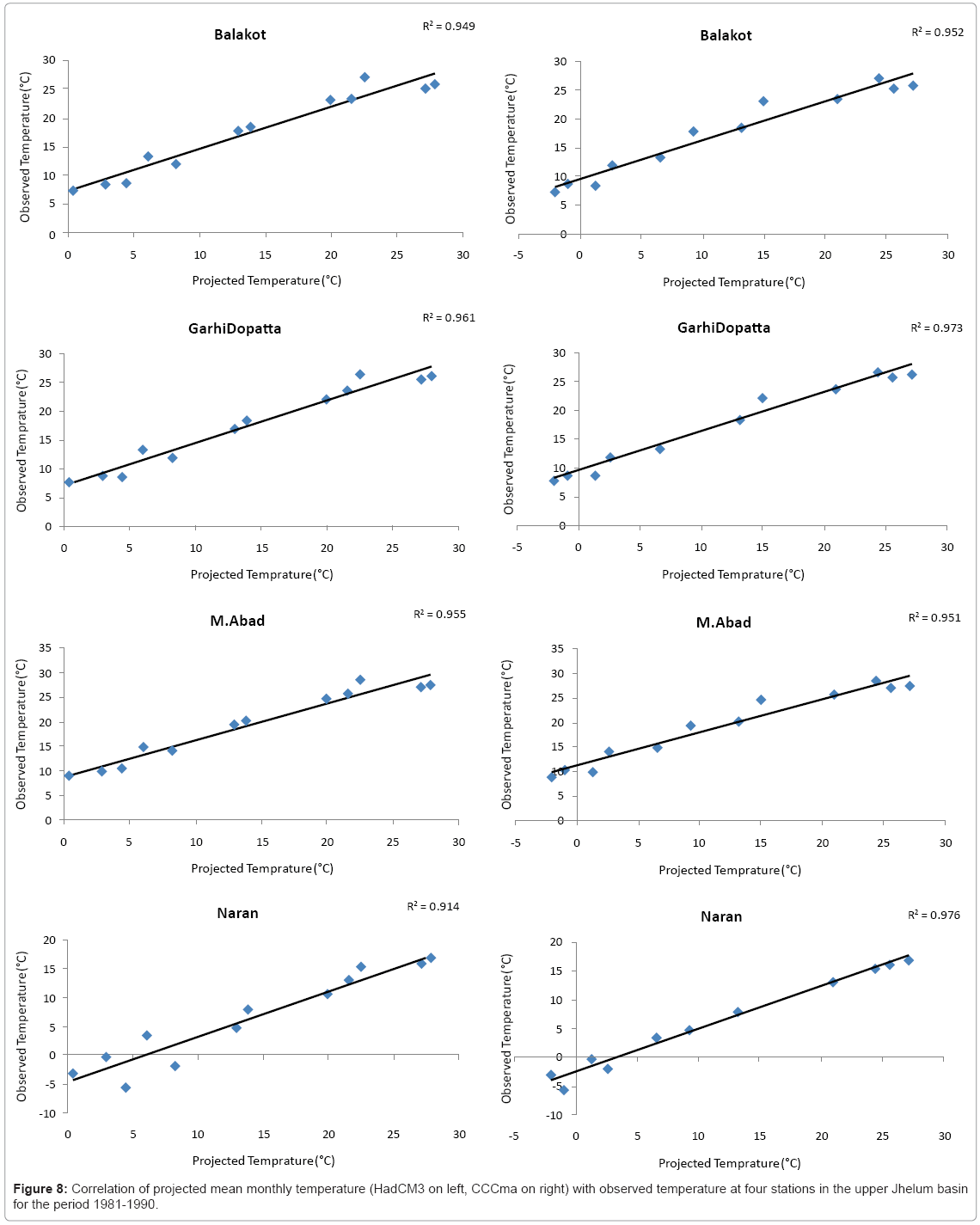
Figure 8: Correlation of projected mean monthly temperature (HadCM3 on left, CCCma on right) with observed temperature at four stations in the upper Jhelum basin for the period 1981-1990.
To produce a probabilistic assessment of potential climate change for the 21st century, CCCma, CSIRO, SRNIES, and HadCM3 models were used for the study area, based on the statistical parameters (Table 3 and Table 4). Figure 9 compares Probability Density Functions (PDFs) of the precipitation and temperature averaged across four stations for the control and future periods. Comparison of the scenario and control PDFs shows a significant shift of the mean to the right of the distribution for temperature, suggesting an increase in annual mean temperature, while in case of precipitation the shift of the mean varies from scenario to scenario.
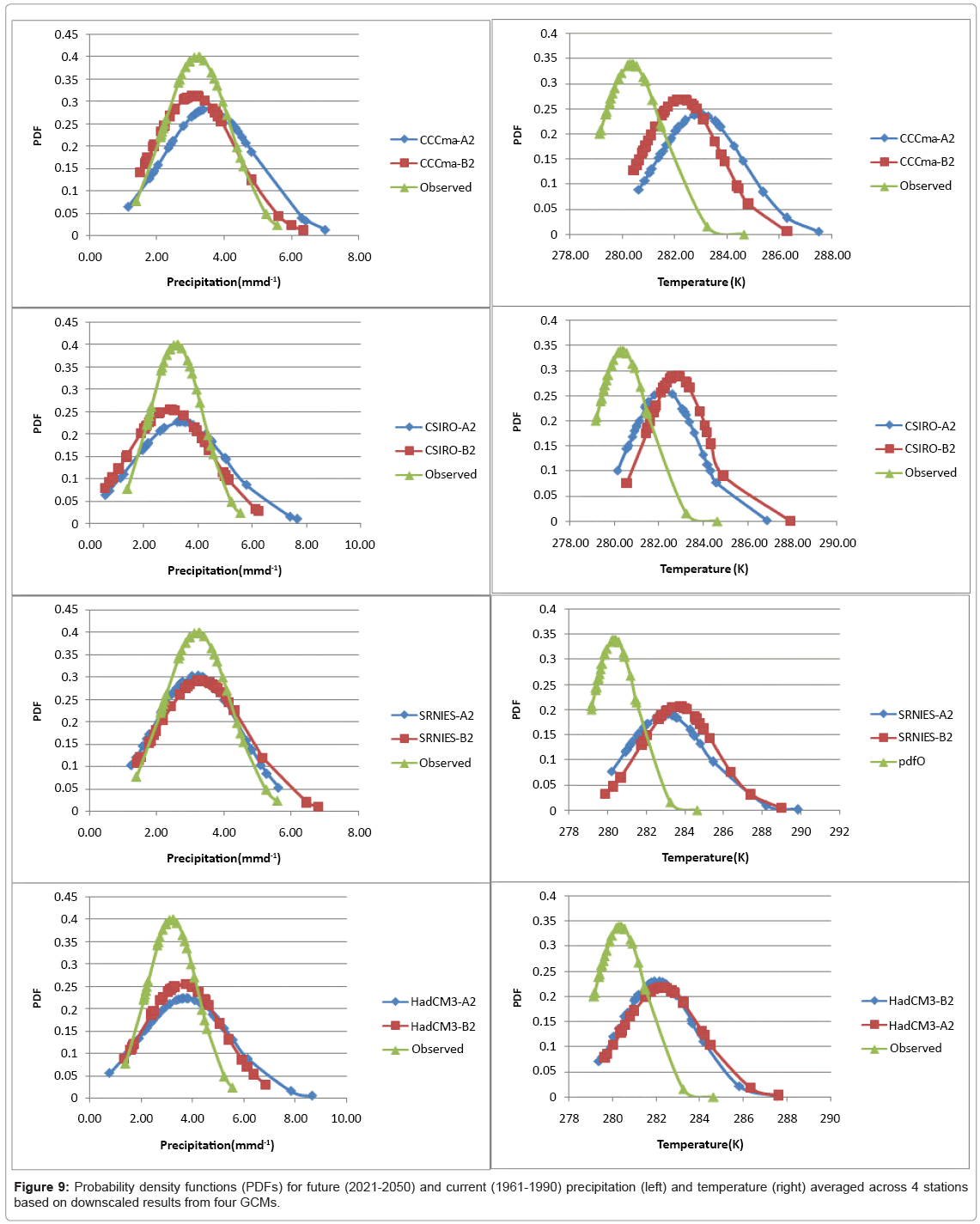
Figure 9: Probability density functions (PDFs) for future (2021-2050) and current (1961-1990) precipitation (left) and temperature (right) averaged across 4 stations based on downscaled results from four GCMs.
An annual time series for the period 2021-2050 is computed for the corresponding grid of HadCM3 to project the future climate scenarios for four stations in upper Jhelum basin. The time series of simulated mean annual temperature and precipitation anomalies, relative to 1961-1990 is presented in Figure 10. For both the scenarios of HadCM3, in case of temperature almost uniform increasing trend is presented at all the stations, while in case of precipitation the trend is inconsistent but an overall increase can be seen at all the stations. Features of climate change across the upper Jhelum basin on annual scale can be seen in Table 5.
| Station | Period | Temperature (°C) | Precipitation (%) | ||
| A2 | B2 | A2 | B2 | ||
| Balakot | 2021-2050 | 1.8 | 1.6 | 2 | 10 |
| Garhi Dopatta | 2021-2050 | 1.9 | 1.7 | 3 | 10 |
| Muzaffar Abad | 2021-2050 | 1.9 | 1.7 | 3 | 10 |
| Naran | 2021-2050 | 1.9 | 1.7 | 10 | 8 |
Table 5: Projected annual mean precipitation (%) and temperature (°C) changes relative to 1961-1990, under A2 and B2 scenarios of HadCM3 at four stations in upper Jhelum basin.
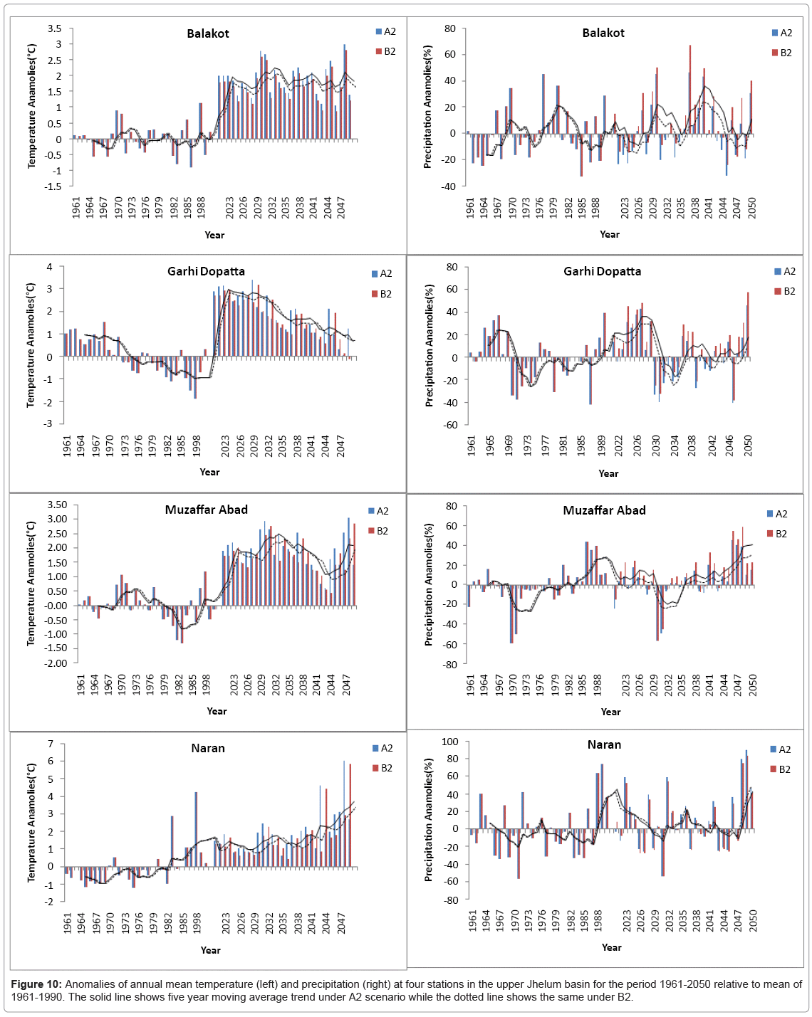
Figure 10: Anomalies of annual mean temperature (left) and precipitation (right) at four stations in the upper Jhelum basin for the period 1961-2050 relative to mean of 1961-1990. The solid line shows five year moving average trend under A2 scenario while the dotted line shows the same under B2.
Conclusion
The developed tool is a Window-based decision support tool for the selection of suitable GCM based on statistical parameters, obtaining different GCMs data in user friendly format such as Excel datasheet, projection of future climate scenarios using delta change technique. The existing tools used for downscaling (e.g. SDSM) do not provide the facility to get GCM data for different models and to project future scenario. Like other downscaling techniques this method also shows good result in case of temperature but in case of precipitation the performance has been poor. To assess the performance of the tool, four climate stations located in upper Jhelum are used. The results show that the agreement between observations and simulations relies on the GCM data. HadCM3, SRNIES models presents good results while simulating the spatial variability of mean temperature in the upper Jhelum.
The software tool reduces the problem of downloading data from IPCC data distribution Centre, and then converting it to user readable format by using different software tools. At the same time the user can find out the suitable GCM for a specific region on the basis of statistical parameters i.e. R2 and RMSE. The availability of different GCM data give confidence to the user to obtain better results and to assess the uncertainties linked with different GCMs. However some more work is needed regarding the addition of new techniques to the existing tool to allow the user to obtain better result and evaluate the uncertainties associated with delta change technique.
Acknowledgements
I am thankful to my scholarship donor, The Higher Education Commission of Pakistan, and AIT, Thailand for their financial support to conduct my research.
References
- Wentz FJ, Ricciardulli L, Hilburn K, Mears C (2007) How much more rain will global warming bring? Science 317: 233-235.
- Chu JT, Xia J, Xu CY, Singh VP (2010) Statistical downscaling of daily mean temperature, pan evaporation and precipitation for climate change scenarios in Haihe River, China. Theor Appl Climatol 99: 149-161.
- Huang J, Zhang J, Zhang Z, Xu CY, Wang B, et al. (2011) Estimation of future precipitation change in the Yangtze River basin by using statistical downscaling method. Stock Env Res Risk A 25: 781-792.
- Mahmood R, Babel MS (2012) Evaluation of SDSM developed by annual and monthly sub-models for downscaling temperature and precipitation in the Jhelum basin, Pakistan and India. Theor Appl Climatol.
- Solomon S, Qin D, Manning M, Chen Z, Marquis M, et al. (2007) Contribution of Working Group I to the fourth assessment report of the intergovernmental panel on climate change, 2007. Cambridge University Press, Cambridge, UK.
- Zhang XC, Liu WZ, Li Z, Chen J (2011) Trend and uncertainty analysis of simulated climate change impacts with multiple GCMs and emission scenarios. Agric Forest Meteor 151: 1297-1304.
- Elshamy ME, Seiertad IA, Sorteberg A (2009) Impacts of climate change on Blue Nile flows using bias-corrected GCM scenarios. Hydrology and Earth System Sciences 13: 551-565.
- Hewiston BC, Crane RG (1996) Climate downscaling: Techniques and application. Clim Res 7: 85-95.
- Wilby RL, Wigely TML (1997) Downscaling general circulation model output: A review of method and limitations. Progress in Physical Geography 214: 530-548.
- Diaz-Nieto J, Wilby RL (2005) A comparison of statistical downscaling and climate change factor methods: Impacts on low flows in the river Thames, United Kingdom. Climatic Change 69: 245-268.
- Fowler HJ, Blenkinsop S, Tebaldi C (2007) Linking climate change modeling to impacts studies: recent advances in downscaling techniques for hydrological modeling. International Journal of Climatology 27: 1547-1578.
- Tabor K, Williams JW (2010) Globally downscaled climate projections for assessing the conservation impacts of climate change. Ecol Appl 20: 554-565.
- Wilby RL, Charles SP, Zorita E, Timbal B, Whetton P, et al. (2004) Guidelines for use of climate scenarios developed from statistical downscaling methods.
- Hewitson BC, Crane RG (2006) Consensus between GCM climate change projections with empirical downscaling: precipitation downscaling over South Africa. International Journal of Climatology 26: 1315-1337.
- Hayhoe K, Cayan D, Field CB, Frumhoff PC, Maurer EP, et al. (2004) Emissions pathways, climate change, and impacts on California. Proc Natl Acad Sci U S A 101: 12422-12427.
- Shongwe, ME, Landman WA, Mason SJ (2006) Performance of recalibration systems for GCM forecasts for southern Africa. International Journal of Climatology 26: 1567-1585.
- Frost AJ, Charles SP, Timbal B, Francis HSC, Mehrotra R, et al. (2011) A comparison of multi-site daily rainfall downscaling technique under Australian conditions. Journal of Hydrology 408: 1-18.
- Liu Z, Xu Z, Charles SP, Fu G, Liu L (2011) Evaluation of two statistical downscaling models for daily precipitation over an arid basin in China. International Journal of Climatology.
- Liu W, Fu G, Liu C, Charles SP (2012) A comparison of three multi-site statistical downscaling models for daily rainfall in the North Chain Plain. Theor Appl Climatol.
- Yurong Hu, Maskey S, Uhlenbrook S (2012) Downscaling daily precipitation over the Yellow River source region in China: a comparison of three statistical downscaling methods. Theor Appl Climatol.
- Gellens D, Roulin E (1998) Streamflow response of Belgian catchments to IPCC climate change scenarios. Journal of Hydrology 210: 242-258.
- Graham LP (2004) Climate change effects on river flow to the Baltic Sea. Ambio 33: 235-241.
- Middelkoop H, Daamen K, Gellens D, Grabs W, Kwadijk JCJ, et al. (2001) Impact of climate change on hydrological regimes and water resources management in the Rhine Basin. Climatic Change 49: 105-128.
- IPCC (2004) Task Group on data and scenario support for Impact and Climate Analysis (TGICA).
- Carter TR, Hulme M, Lal M (1999) Guidelines on the use of Scenario Data for climate impact and adaptation assessment. Task Group on Scenarios for Climate Impact Assessment Intergovernmental Panel on Climate Change (TGCIA).
- IPPC (2001) Climate Change-Impacts, Adaptation and Vulnerability. Cambridge University Press, Cambridge, UK.
- Arnell NW (1998) Effects of Climate Change on River Flows: Update Using the UKCIP98 Scenarios, in UK Environment Agency. University of Southampton, UK.
- Akhtar M, Ahmad N, Booij MJ (2008) The impacts of climate change on the water resources of Hindukush-Karakorum-Himalaya region under different coverage scenarios. Journal of Hydrology 335: 148-163.
- IPPC (2001) Climate Change 2001: The Scientific Basis. Cambridge University Press, Cambridge, UK.
- Feenstra JF, Burton I, Smith JB, Tol RSJ (1998) Handbook on Methods of Climate Change Impacts and Adaptation strategies. UNEP/IES, Amesterdam, The Netherlands.
- Shahzad MKK (2011) Impacts of climate change on the water resources and irrigation water demand in the upper Indus river basin, Pakistan, in Water Resource and Management. Asian Institute of Technology: Thailand.
Citation: Ullah K, Shrestha, S, Guha S (2012) A Decision Support Tool for Selection of Suitable General Circulation Model and Future Climate Assessment. J Earth Sci Climate Change 3: 117. DOI: 10.4172/2157-7617.1000117
Copyright: ©2012 Ullah K, et al. This is an open-access article distributed under the terms of the Creative Commons Attribution License, which permits unrestricted use, distribution, and reproduction in any medium, provided the original author and source are credited.
Select your language of interest to view the total content in your interested language
Share This Article
Recommended Journals
Open Access Journals
Article Tools
Article Usage
- Total views: 15676
- [From(publication date): 7-2012 - Dec 04, 2025]
- Breakdown by view type
- HTML page views: 10680
- PDF downloads: 4996