An Assessment of Temperature and Precipitation Change Projections using a Regional and a Global Climate Model for the Baro-Akobo Basin, Nile Basin, Ethiopia
Received: 22-Jan-2013 / Accepted Date: 21-Feb-2013 / Published Date: 25-Feb-2013 DOI: 10.4172/2157-7617.1000133
Abstract
In this study, large-scale atmospheric output variables from CGCM3.1 global circulation model and the regional model REMO are downscaled statistically to meteorological variables at the point scale in a daily resolution to assess future climatic variables under climate changes. The area of study is Baro-Akobo river basin in Ethiopia, which contributes to the White Nile in Sudan. The minimum and maximum temperature and precipitation variables were selected, and future time scenarios of these variables were projected based on climate scenarios of A1B and B1 for a period of 2011 to 2050.Both REMO and CGCM3.1 outputs capture the observed 20th century trends of temperature and precipitation change over the basin. However, the result of downscaled precipitation reveals that precipitation does not verify a systematic increase or decrease in all future time horizons for both A1B and B1 scenarios unlike that of maximum temperature. For REMO A1B and B1 scenarios similar trend +1.3°C changes for maximum temperature are expected, and rainfall increases as much as 24% for the 2011 to 2050 period. For the CGCM3.1 model +2.55°C changes in maximum temperature and 23% increase in rainfall is likely.
Keywords: Climate change; Statistical downscaling; REMO; CGCM
9483Introduction
Climate change impact studies associated with global warming as a result of Green House Gases (GHG) has been given ample attention worldwide in the recent decades because of perceived impact on global, regional as well as local socio-economic, livelihood and natural resources. According to the Intergovernmental Panel on Climate Change (IPCC) 4th assessment report [1] global average surface temperature would likely rise between 2°C to 4.5°C by 2100 with the doubling of atmospheric carbon dioxide (CO2). For the continent of Africa [2], the warming during this century would very likely be larger than the global average (3°C). With respect to precipitation, the results are different for different regions; the report also indicates that an increase in mean annual rainfall in East Africa is likely. The minimum temperature over Ethiopia show an increase of about 0.37°C per decade, which indicates the signal of warming over the period of the analysis 1957-2005 [3]. Previous studies in Nile basin provide different indication regarding long term rainfall trends; Elsahmay et al. [4] reported future precipitation change in the Blue Nile is uncertain in their assessment of climate change on stream flow of the Blue Nile for 2081-2098 period using 17 GCMs. Wing et al. [5] showed that there are no significant changes or trends in annual rainfall at the national or watershed level in Ethiopia; Taye et al. [6] reported impact of climate change on rainfall trend is unclear for the Lake Tana catchment (Blue Nile part) while for Nyando River (White Nile part) rainfall shows increasing trend under two future SRES emission scenarios A1B and B1 for 2050s. Beyene et al. [7] showed that the Nile River is expected to experience an increase in stream flow early in the study period (2010- 2039), due to generally increased precipitation; it is expected to decline during mid (2040-2069) and late (2070-2099) century as a result of both precipitation declines and increased evaporative demand. Furthermore, Conway [8], Elsahmay et al. [4], Yimer et al. [9] also reported about uncertainty of the direction and magnitude of future changes in rainfall whilst temperature are expected to increase. Therefore previous studies show that many parts of the Nile are sensitive to climate change and it has a prospective impact on the water resources in the area. However, the climatic regions of the Nile are variable and dividing the basin into different regions and sub-basin will be a convincing and proficient approach when studying impacts of climate change [6].
Generally, climate change scenarios are coarse in resolution may not be directly applied to local scale studies to understand the likely impact of the climate change. This study mainly focuses on the impact of climate change on the hydrology of a river basin scale at local scale application. It is widely accepted that Atmospheric-Ocean General Circulation Models (GCMs) are the best physically based means for predicting future climate [10]. Despite the fact that the impact of climate change scenarios forecasted at a global scale, their coarse spatial resolution may not be used directly for studies at a small watershed scale. Dibike et al. [11] reported a clear need for high resolution scenarios at a spatial scale much finer than that provided by a global or even some regional climate models. Consequently, as Yimer et al. [9] described downscaling techniques emerged as a means to relate the scale mismatch between the GCMs and the small scales required at watershed level. The main downscaling approaches frequently used in development of higher resolution climate scenarios are dynamical and statistical downscaling [9,11,12]. Dynamical downscaling generates regional or local scale climate scenario data by developing and using Regional Climate Models (RCMs) with the coarse GCM data used as boundary conditions. Statistical Down-Scaling Method (SDSM) on the other hand involves developing quantitative relationships between large scale atmospheric variables, the predictors, and local surface variables, the predictands.
The focus of this study it to provide first-hand understanding of the direction of climate change in one of the remote basins of Ethiopia (Baro-Akobo basin) where there is little previous research work on likely impact of climate change. The basin is one of a productive agricultural area and covers a higher percentage of natural forest than the rest of the country. The objective of the study is assessing temperature and rainfall change projection from CGCM3.1 and REMO using downscaling techniques within the Baro-Akobo basin for a period of 2011-2050.
Approaches for climate downscaling
This section briefly summaries the various downscaling approaches available in the literature. Although the GCMs’ ability to reproduce the current climate has increased, direct outputs from GCM simulations are inadequate for assessing hydrological impacts of climate change at regional and local scales [13]. Indeed, many hydrological impact assessments need station/point scale climate variables; therefore there is a clear need for reliable high resolution scenarios at station scale finer than that of GCMs performed through downscaling. Two downscaling approaches that are commonly used for climate scenario development are dynamical downscaling and statistical downscaling.
In the dynamical downscaling approach a Regional Climate Model (RCM) is nestled into a GCM were GCMs are used to fix boundary conditions. The major disadvantage of dynamical downscaling in climate impact study is its high computational and technical demands at the outset [14]. Statistical Downscaling (SD) involves developing quantitative relationships between large-scale atmospheric variables and local-scale surface variables, since SD is derived from the historical observed data, it provide site specific information as recommended in many climate change impact studies [11,15].
The most common SD approaches are namely; Statistical Down- Scaling Model (SDSM), Long Ashton Research Station Weather Generator (LARS-WG) and Artificial Neural Network (ANN). SDSM is a hybrid of a stochastic weather generator and multiple regression based method [16]. During downscaling with SDSM a multiple linear regression model is developed between a few selected large-scale predictor variables and local scale predictands such as precipitation and temperature [11,17]. As Yimer et al. [9] described Predictor is input data used in SDSM, typically a large scale variable describing the circulation regime over a region, it is also known as “independent variable”, or simply as the “input variable”. The predictand is the output data, typically the small-scale variable representing temperature or precipitation at a weather/climate station.
SDSM can be used to provide local information, which could be used in many climate change impact assessment. It is computationally inexpensive and thus can be easily applied to the output of different GCM experiments [18]. According to Wilby and Wigley [19] in SD the following assumptions are made in order to use such type of downscaling methods for assessing climate change (i) appropriate relationships can be developed between large scale and small scale grid predictor variables; (ii) these observed empirical relationships are valid also under climate change conditions; and (iii) the predictors variables and their change are well characterised by GCMs. If these assumptions hold, it is then possible to produce climate scenarios of regional and small scale with finer resolution and more reliable than raw GCMs from future climate change data produced by GCMs.
In LARS-WG, for precipitation downscaling, observed daily local station precipitation of each month are analysed using a number of years of historical data to obtain statistical characteristics such as number of dry days, wet days and mean daily precipitation in each month of a year. This information is used to develop semi-empirical distributions for the lengths of wet and dry day series and daily precipitation amount, the precipitation value is generated from the semi-empirical precipitation distribution. On the other hand ANN is a non-linear regression type in which a relationship is developed between a few selected large-scale atmospheric predictors and basin scale meteorological predictands [20].
Compared with dynamic downscaling, SD methods have the following advantages [13]: (i) based on standard and accepted statistical procedures, (ii) computationally inexpensive, (iii) may be flexibly crafted for specific purpose, (iv) able to directly incorporate the observational record of the region. Wilby and Dawson [14] reports a number of studies show that SDSM yields reliable estimates of extreme temperatures, seasonal precipitation totals, areal and intersite precipitation behaviour. Thus we applied the program SDSM 4.2 [18] for this study to downscale the outputs of REMO and CGCM for Baro-Akobo basin. Furthermore, there is little study on climate change in Baro-Akobo basin and this study may form one of the first understandings of the direction of climate change.
The organization of this paper is as follows; the next section continues with description on scenarios used for downscaling approaches. Study area and data used in this study are described in part two. In part three ‘methodology’ methods used in the analysis presented, results are shown and discussed in part four ‘Results and discussion’ while conclusion and some remarks are given in part five entitled ‘conclusion’.
Scenarios used
The IPCC developed scenarios that have been widely used in the analysis of possible climate change and options to mitigate, among these A1B and B1 scenarios were used in this study. A1B scenario belongs to A1 family that describes a future world of very rapid economic growth and rapid introduction of new and more efficient technologies. A1B group is distinguished by balanced across all sources of energy not relaying on one particular source, on the assumption that similar improvement rates apply to all energy supply and end use technologies. Whereas the B1, scenario describes rapid change in economic structures towards a service and information economy, with reductions in material intensity and the introduction of clean and resource-efficient technologies [2].
REMO: The regional climate model REMO is a hydrostatic, threedimensional atmospheric model that has been developed in the context of the Baltic Sea Experiment (BALTEX) at the Max-Planck-Institute for Meteorology in Hamburg1. It is based on the Europa Model (EM), the former numerical weather prediction model of the German Weather Service (DWD) and is described in Jacob [21]. Additionally, the physical parameterization package of the general circulation model ECHAM4 has been implemented. Physical parameterizations are taken from ECHAM4 and adjusted to the scale of REMO [22]. Further detailed information on the REMO development and model characteristics can be found at http://www.remo-rcm.de/REMO-Model-Characteristics.1 268+M54a708de802.0.html.
In the present version, the model is run at 0.5° horizontal resolution with 20 terrain-following vertical levels. The model domain covers the entire tropical and northern parts of Africa from 30°W to 60°E and from 15°S to 45°N [23]. The model considers land use change for both A1B and B1 scenarios and also it has ensemble runs for A1B without land use change. The REMO model which covers the area of interest (5 to 11°N and 33 to 37°E) with land use change was used in this study. The basin is covered by 50 REMO raster nodes (Figure 1). Among these are 17 REMO nodes near climate/meteorological stations used for downscaling. The predictor variables used for downscaling REMO are precipitation, maximum and minimum temperature, radiation and relative humidity data of REMO grid cells surrounding each meteorological station.
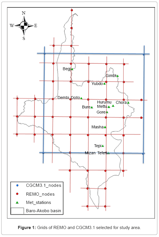
Figure 1: Grids of REMO and CGCM3.1 selected for study area.
CGCM3.1: CGCM3.1 is the third version of Canadian Coupled Global Climate Models (CGCM3.1) and shares many basic features with the second generation model as described in McFarlane et al. [24] and Scinocca et al. [25]. Further detailed information on CGCM3.1 development and model characteristics can be found at (http:// www.ec.gc.ca/ccmac-cccma/default.asp?lang=En&n=89039701-1). Predictor data files or SDSM inputs from CGCM3.1 and NCEP (National Centre for Environmental Prediction) were extracted from the Data Access Integration (DAI) [26] website (http://loki.ouranos. ca/DAI/gcm-e.html); which is an online climate and environmental data distribution tool. The predictor variables for CGCM3.1 (Third generation of the Canadian Coupled Global Climate Model) were provided on a grid box by grid box basis of size correspond and to the value over the centre of the cell defined an area of a 3.75° longitude and 3.75° latitude. The NCEP/NCAR (National Centre for Atmospheric Research) reanalysis products have been interpolated onto the CGCM3 grid, and made available for the calibration procedure of SDSM over the base period (1961-2001). The study area Baro-Akobo basin lies in four CGCM grid nodes [9.28° Lat 33.75°Lon, 5.57° Lat 33.75°Lon, 9.28° Lat 37.5° Lon and 5.57° Lat 37.5° Lon] (Figure 2), from these grid nodes 25 large scale atmospheric variables2 were extracted and used as potential inputs to SDSM.
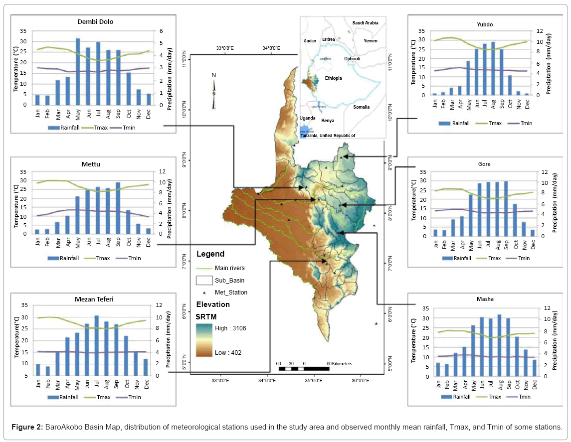
Figure 2: BaroAkobo Basin Map, distribution of meteorological stations used in the study area and observed monthly mean rainfall, Tmax, and Tmin of some stations.
Study Area and Data Used in this Study
Baro-Akobo Basin lies in the southwest of Ethiopia between latitudes of 5° 31` and 10° 54` N, and longitudes of 33° 0` and 36° 17` E. The basin area is about 76,000 km2 and is bordered by the Sudan in the West, northwest and southwest, Abbay and Omo-Ghibe Basins in the east (Figure 3). The major rivers within the Baro-Akobo basin are Baro and its tributaries Alwero, Gilo and the Akobo. These rivers, which arise in the eastern part of the highlands, flow westward to join the White Nile in Sudan. The mean annual runoff of the basin is estimated to be about 23 km3 as gauged at Gambela station.
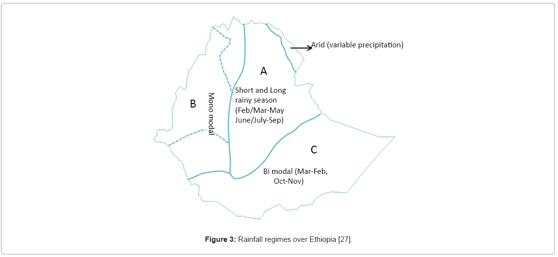
Figure 3: Rainfall regimes over Ethiopia [27].
Elevation of the study area varies between 440 and 3000 m a.m.s.l. The higher elevation ranges are located in the North East and Eastern part of the basin while the remaining part of the basin is found in lower elevation. In the study area, there is high variability in temperature with large differences between the daily maximum and minimum temperatures. Figure 1 shows that large temperature differences can be observed by the catchment topographic settings where temperature decreased with increase in altitude.
Climate station data (Predictands)
Data used in the study are daily rainfall, maximum and minimum temperature collected and archived by the Ethiopian National Meteorological Agency (NMA) from 12 stations in and around the Baro-Akobo river basin, from 1972 to 2000 in general. The choice was forced by data extent and the sparse station network in the basin. The number of meteorological stations and extent of data used in downscaling experiment are depicted in Table 1.
| Station | Elevation (m) | Lat (degree) | Lon (degree) | Precipitation (mm) | Maximum Temperature(°C) | Minimum Temperature(°C) |
|---|---|---|---|---|---|---|
| Tepi | 1230 | 7.20 | 35.42 | 1981-2000 | 1981-2000 | 1981-2000 |
| MezanTeferi | 1400 | 7.00 | 35.58 | 1987-2000 | 1982-1991 | 1982-1991 |
| DembiDollo | 1550 | 8.53 | 34.80 | 1979-2000 | 1979-2000 | 1979-2000 |
| Yubdo | 1560 | 8.95 | 35.45 | 1976-2000 | 1976-2000 | 1976-2000 |
| Mettu | 1690 | 8.30 | 35.58 | 1976-2000 | 1976-2000 | 1976-2000 |
| Bure | 1700 | 8.28 | 35.10 | 1976-2000 | 1976-2000 | 1976-2000 |
| Begi | 1722 | 9.35 | 34.53 | 1979-2000 | 1978-2000 | 1978-2000 |
| Hurumu | 1800 | 8.33 | 35.70 | 1973-2000 | - | - |
| Chora | 1930 | 8.42 | 36.13 | 1975-2000 | - | - |
| Gimbi | 1970 | 9.17 | 35.80 | 1978-2000 | 1979-1993 | 1979-1993 |
| Gore | 2024 | 8.15 | 35.53 | 1972-2000 | 1972-2000 | 1972-2000 |
| Masha | 2200 | 7.73 | 35.48 | 1975-2000 | 1980-1999 | 1980-1999 |
Table 1: Metrological stations and data periods used in the study area.
In Ethiopia, as shown in the Figure 3, the pattern and character of rainfall varies in different parts of the country. There are some regions which experience three seasons (tri-modal type, region A) with two rainfall peaks (where one peak is more prominent than the other), while some regions have four seasons with two distinct rainfall peaks (bi-modal type, region C). There are still some regions, which have two seasons with a single rainfall peak (mono-modal type, region B). The Area under region B is where the Baro-Akobo basin lies and is characterized by a single rainfall peak during a year, with two distinct seasons, one being wet (rainy season) locally called “Kiremt” and the other dry called “Bega”.
Mean monthly rainfall pattern shows that the south-western and western part of the country in region B is under the wet season during February/March to October/November and April/May to October/November respectively. Therefore, stations Tepi, Mezan Teferi and Masha belong to the Bega (December, January and Feberuary) and Kiremt (March to October) seasons and are named as southern part of the basin here after. Whereas stations Gore, Bure, Yubdo, Dembi Dollo, Gimbi, Mettu, Begi and Assosa are in Bega season (November, December, January and February) and will be in Kiremt season (May to October) and named as Northern part of the basin here after for the purpose of looking at seasonal climate change in the area.
Methodology
Downscaling
SDSM 4.2.2 statistical downscaling model was supplied on behalf of the Environment Agency of England and Wales. It is a decision support tool used to asses local climate change impacts using a SD technique. The software manages additional tasks of data quality control and transformation, predictor variable pre-screening, automatic model calibration, basic diagnostic testing, statistical analysis and graphing of climate data. SDSM [16] is best described as a hybrid of stochastic weather generator and regression-based methods. Through downscaling using SDSM, multiple regression models were developed between selected large-scale predictor variables (NCEP/NCAR), (REMO) and local scale predictands. The parameters of the regression equation are estimated using an ordinary Least Squares algorithm. Precipitation is modeled as a conditional process in which the local precipitation amount is correlated with the occurrence of wet days. As the distribution of precipitation is skewed, a forth root transformation is applied to the original series to convert it to the normal distribution, and then used in the regression analysis. Minimum and maximum temperatures are modeled as unconditional process, where a direct link is assumed between the large scale predictors and local scale predictand. Additionally, stochastic techniques are used to artificially inflate the variance of the downscaled daily time series to better accord with observations.
One of the challenging stages in SD is the choice of appropriate predictor variable(s), this is due to the fact that downscaling is highly sensitive to the choice of predictor variables, and also decision on predictor variables determines the character of the downscaled climate scenario. Beside this the explanatory power of individual predictor variables varies spatially and temporally [18]. Screening of the most appropriate predictor variables was carried out through the percentage of explained variance analysis, linear correlation analysis, partial correlation analysis, and scatter plots between predictor and predictand variables. SDSM normally calibrated by a linear regression based on NCEP/NCAR reanalysis data and station data then later applied to GCM data. For this study, large-scale NCEP/NCAR predictor variables representing the current climate condition were used for analysis subsequently applied to CGCM3.1. Table 2 shows the selected predictor variables from NCEP/NCAR for each meteorological station in the downscaling procedure. Whereas for downscaling REMO, SDSM calibrated using precipitation, maximum temperature, minimum temperature, wind, radiation, and relative humidity data of each stations served as predictands, while the surrounding grid cells of REMO for the same variable of each climate model served as predictor variables.
| Station | Predictand | Predictors* | |||||
|---|---|---|---|---|---|---|---|
| Tepi | Temperature max | ncepp_thaf | Nceptempaf | ||||
| Temperature min | ncepp_vaf | ncepp_zaf | Ncepp850af | Nceps850af.dat | |||
| Rainfall | Ncepp8zhaf | Nceps850af | |||||
| MezanTeferi | Temperature max | ncepp_thaf | Ncepp8_uaf | Ncepp8thaf | Nceptempaf | ||
| Temperature min | ncepp_vaf | Ncepp500af | Nceps850af | Nceptempaf | |||
| Rainfall | ncepp_zaf | Ncepp5thaf | Ncepp8zhaf | ||||
| DembiDollo | Temperature max | ncepp_thaf | Ncepp5_zaf | Nceptempaf | |||
| Temperature min | Ncepp8_faf | Ncepp850af | |||||
| Rainfall | Ncepp8_uaf | Nceptempaf | |||||
| Yubdo | Temperature max | ncepp_thaf | Ncepp5_zaf | Ncepp8thaf | Nceptempaf | ||
| Temperature min | ncepp_vaf | Ncepp500af | Nceps850af | Nceptempaf | |||
| Rainfall | ncepp_zaf | Ncepp5thaf | Ncepp8zhaf | Nceps850af | |||
| Mettu | Temperature max | Ncepp5_zaf | Ncepp8thaf | Ncepp8zhaf | Nceptempaf | ||
| Temperature min | ncepp_thaf | Ncepp5_zaf | Ncepp8thaf | Nceptempaf | |||
| Rainfall | ncepmslpaf | Ncepp5thaf | Nceps850af | ||||
| Bure | Temperature max | ncepp_zaf | ncepp_thaf | Ncepp5thaf | Ncepp8thaf | Nceptempaf | |
| Temperature min | ncepp_uaf | Ncepp5thaf | Nceptempaf | ||||
| Rainfall | ncepp_thaf | Ncepp5thaf | Ncepshumaf | ||||
| Begi | Temperature max | ncepp_thaf | Ncepp5_zaf | Nceptempaf | |||
| Temperature min | ncepp_vaf | Ncepp500af | |||||
| Rainfall | ncepp_zaf | Ncepp5_zaf | |||||
| Hurmu | Temperature max | ||||||
| Temperature min | |||||||
| Rainfall | Ncrpp8zhaf | nceptempaf | |||||
| Chora | Temperature max | ncepp_thaf | Nceptempaf | ||||
| Temperature min | Ncepp8_faf | Nceps850af | Nceptempaf | ||||
| Rainfall | ncepp_zaf | Ncepp_zhaf | |||||
| Gimbi | Temperature max | ncepp_thaf | Ncepp8thaf | Nceptempaf | |||
| Temperature min | ncepp_vaf | ncepp_thaf | Nceptempaf | ||||
| Rainfall | ncepp_faf | Ncepp8zhaf | |||||
| Gore | Temperature max | ncepp_faf | ncepp_thaf | ncepp_zhaf | Ncepp5thaf | Ncepp8thaf | Nceptempaf |
| Temperature min | Ncepp5thaf | Ncepp8thaf | Nceptempaf | ||||
| Rainfall | ncepp_zaf | ncepp_zhaf | Nceps500af | ||||
| Masha | Temperature max | ncepp_faf | Ncepp5_vaf | Ncepp8thaf | Nceptempaf | ||
| Temperature min | ncepp_zaf | Ncepp5_uaf | Ncepp8_vaf | Nceptempaf | |||
| Rainfall | Ncepp8zhaf | Nceps850af | |||||
Description of each predictor variables indicated in Table 2*
| Predictors | Description | Predictors | Description |
| ncepp_faf.dat | 10_WS | Ncepp5zhaf.dat | 5_Di |
| ncepp_vaf.dat | 10_MWC | Ncepp8_faf.dat | 8_WD |
| ncepp_zaf.dat | 10_Vor | Ncepp8_uaf.dat | 8_ZWD |
| ncepp_thaf.dat | 10_WD | Ncepp8_vaf.dat | 8_MWC |
| ncepp_zhaf.dat | 10_Di | Ncepp850af.dat | 8_Gp |
| Ncepp5_zaf.dat | 5_WD | Ncepp8thaf.dat | 8_WD |
| Ncepp5_uaf.dat | 5_ZWC | Ncepp8zhaf.dat | 8_Di |
| Ncepp5_vaf.dat | 5_MWC | Nceps500af.dat | 5_SH |
| Ncepp5_zaf.dat | 5_Vor | Nceps850af.dat | 8_SH |
| Ncepp500af.dat | 5_Gp | Ncepshumaf.dat | 10_SH |
| Ncepp5thaf.dat | 5_WD | Nceptempaf.dat | Temperature @ 2m |
Where: WS= wind speed; MWC= Meridional wind component; Vor=vorticity; Wd=wind direction; Di=divergence; ZWC= zonal wind component; Gp= Geoptential; SH=Specific humidity; 10_=1000hpa; 8_=850hpa; 5_=500hpa
Table 2: Predictors selected for model calibration at different station.
Ensemble simulation
The advantage of using SD is the possibility of generating statistical ensembles. An ensemble is a large (possible infinite) number of copies of a system, considered all at once, each of which represents a possible state that the real system might be in at some specified time [28]. Depending on the total number of simulations conducted, ensemble forecast analyses range from simply averaging forecasts and evaluating their variability using bounding boxes to much more sophisticated approaches analyzing the probabilities of forecasts [29]. For this study 20 ensembles were generated using the model and used to examine the precipitation and temperature change in Baro-Akobo basin. SDSM have the capacity to generate up to 100 ensembles and can be used to research the uncertainty analysis of climate scenario. Due to the computational capacity of the hydrological models subsequently to be used after downscaling and storage required we were forced to restrict the number of ensembles to 20 for each climate models (REMO and CGCM3.1) and each scenario A1B and B1.
Calibration and validation
Model calibration was done based on the selected predictor variables that were derived from the REMO and NCEP/NCAR data set. Calibration in this case aims to find the coefficients of the multiple regression equation parameters that relate the climatic variables derived from REMO, NCEP/NCAR and local scale variables. SDSM has the possibility of finding annual, seasonal and monthly regression functions to downscale the meteorological variables. For this study the temporal resolution of the downscaling model was specified as monthly for the entire stations because the correlation between the data produced by the meteorological stations and the grid cell prediction was found to be good for the purpose.
Model setup parameters like event threshold, bias correction and variance inflation were adjusted during calibration to obtain best statistical agreement between the observed and simulated climate variables. During the calibration of precipitation: daily and monthly mean, variance, QQ-plot, PDF plot, dry and wet-spell lengths were used as performance criteria. The stochastic component of SDSM allows for performing 100 ensembles in the validation process. In this study 20 ensembles are performed, and the average of the twenty independent stochastic GCM ensembles was taken for analysis. The model developers Wilby et al. [17] suggested that, as the target here is only to see the general trend of the climate change in the future; it is adequate to consider the average of the ensembles. They also added that to preserve inter-variable relationships, the ensemble mean should be used.
Climate change scenario
The base line data for the base period were from 12 stations in and around the Baro-Akobo basin within the range of 29 to 14 years period from 1972-2000 and 1987-2000 respectively. Accordingly REMO and CGCM3.1 was downscaled for two emission scenarios (A1B and B1 for REMO and A1B for CGCM3.1) this is because NCEP/NCAR has no predictor variables for the B1 scenario. The first 18 (1972-1989)to 8 (1987-1994) years of data were considered for calibrating SDSM while the remaining 11 to 6 years (1990-2000) to (1995-2000) respectively, were used for validation. Beside graphical fit, the statistical analyses were used to compare downscaled data and base period observation. The performance of the model during the calibration and validation period and the climate change scenario results are explained in the following section.
Results and Discussion
For all stations, downscaled base-line daily temperature data shows good agreement with observation for both calibration and validation periods. In case of daily precipitation even though there were little variations in individual months the performances of the model overall shows a good agreement between the observed and calibrated for almost all months of the year. Figures 4-6 shows the performance of the models during calibration/downscaled period and the original REMO/ CGCM3.1 data before downscaling. As depicted in the figures (Figures 4-6) despite the discrepancyin the values, the skill of both models in capturing the seasonal pattern of both the temperature and rainfall makes the models a good choice for the region. It is also important to recognize the improvement in the outputs of the statistical downscaling can also attributed to the good skill of the REMO/CGCM3.1 model in the region. Unlike temperature, precipitation is a conditional process that depends on other physical intermediate processes like occurrence of humidity, cloud cover, and /or wet-days and the accuracy of downscaling precipitation is less consistent as anticipated mainly due to the obvious complex physical processes and intermediate processes that may not be captured by statistical downscaling.
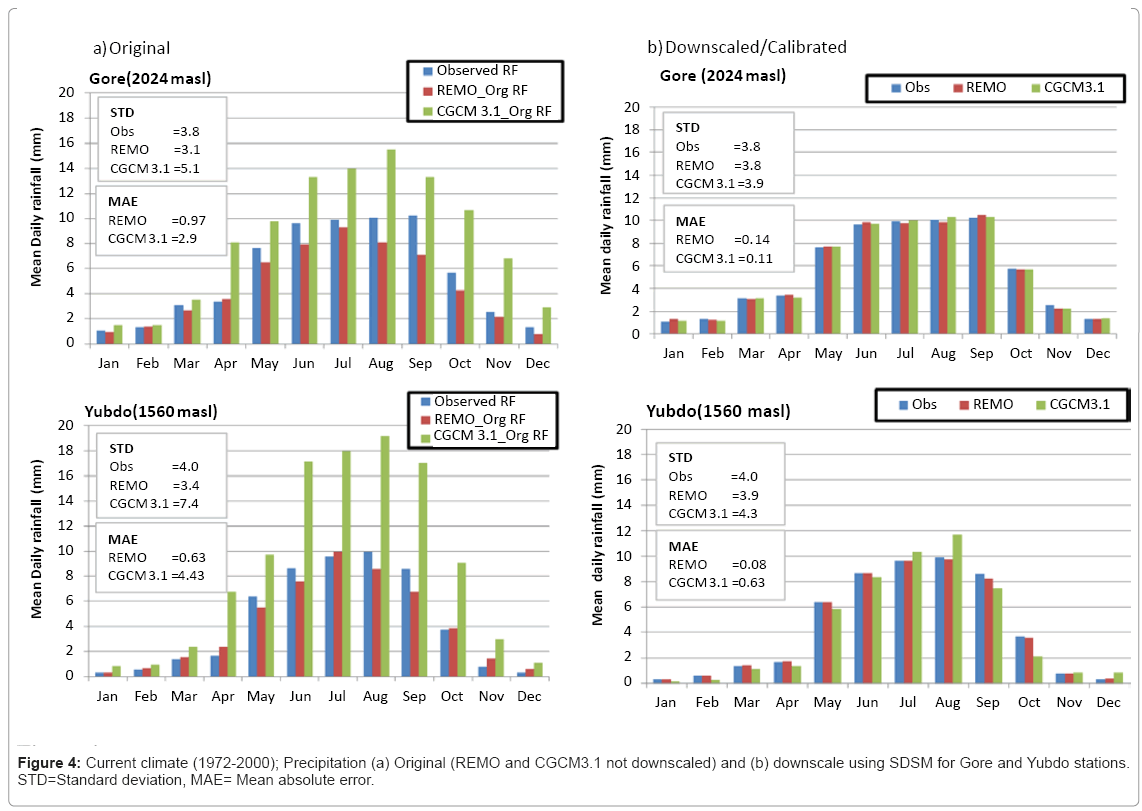
Figure 4: Current climate (1972-2000); Precipitation (a) Original (REMO and CGCM3.1 not downscaled) and (b) downscale using SDSM for Gore and Yubdo stations. STD=Standard deviation, MAE= Mean absolute error.
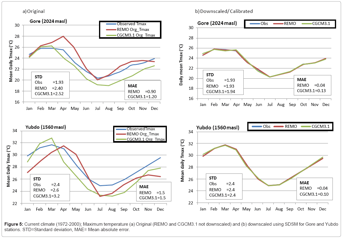
Figure 5: Current climate (1972-2000); Maximum temperature (a) Original (REMO and CGCM3.1 not downscaled) and (b) downscaled using SDSM for Gore and Yubdo stations. STD=Standard deviation, MAE= Mean absolute error.
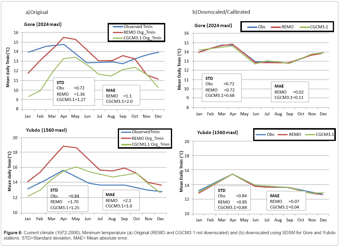
Figure 6: Current climate (1972-2000); Minimum temperature (a) Original (REMO and CGCM3.1 not downscaled) and (b) downscaled using SDSM for Gore and Yubdo stations. STD=Standard deviation, MAE= Mean absolute error.
Generally, results of downscaling for both climate model reveals that all stations considered in this study show good agreement with the observed data.
To examine the performance of the climate models, observed and downscaled values of the base period were averaged to mean annual rainfall, and rainy days were calculated (Table 3). The result shows mean annual rainfall and rainy days partly captured by both models REMO and CGCM3 (Table 3).
| Stations(altitude) | Original Observation / Model run | Mean Annual (mm) | Rainy days (days/year) |
|---|---|---|---|
| Gore (2024 masl) | Observation | 2035 | 170 |
| REMO | 2033 | 176 | |
| CGCM3.1 A1B | 2012 | 179 | |
| Bure (1700 masl) | Observation | 1283 | 153 |
| REMO | 1213 | 154 | |
| CGCM3.1 A1B | 1393 | 144 | |
| Chora (1930 masl) | Observation | 1648 | 135 |
| REMO | 1690 | 138 | |
| CGCM3.1 A1B | 1992 | 181 | |
| Yubdo(1560 masl) | Observation | 1474 | 120 |
| REMO | 1538 | 145 | |
| CGCM3.1 A1B | 1631 | 128 |
Table 3: Comparison of base period (observed and downscaled) annual rainfall and rainy days values for station Gore, Bure, Chora and Yubdo.
Downscaling future scenario
After calibrating the model, the empirical relationships created between the large scale predictor and local scale variables were applied to downscale the future climate change scenario. Twenty ensembles of synthetic daily time series for the period of 40 years (2011-2050) were generated for A1B and B1 SRES emission scenarios. The period 201-2050 aggregated to20 years for future trend comparison from base year for REMO and CGCM3.1. The following section shows projected change of rainfall, maximum and minimum temperature annually and seasonally for stations considered in the study area.
Maximum temperature: As depicted in Figure 7, it can be seen that generally increasing annual trend is likely for maximum temperature in all stations except Gore for both A1B and B1 scenario of REMO. Statistically downscaled REMO results show that there might be a general incremental trend of maximum temperature for A1B and B1 scenario for the period of 2011-2030 and 2031-2050 in the range of +0.1°C to +1.23°Cand +0.1°C to +1.3°C respectively. However, stations Masha, Bure and Mettu show almost no change. It is also noted that the projected change appears to show generally increasing trend with decreasing altitude in the basin (Figure 8 and 9) In case of CGCM3.1 A1B scenario, generally increasing annual trend is expected for the period of 2011-2030 and 2031-2050 in the range of +0.2°C to +2.52°C and +0.1°C to +2.55°C respectively. However, the decreasing annual trend Bure, Begi, Gimbiand Tepi stations may be associated to the problem of downscaling from Global models. We don’t think the results are correct, however, the basin wide temperature increase is evident even with this mode. Therefore, the A1B scenario of REMO and CGCM3.1 agrees for most stations with the direction of maximum temperature change.
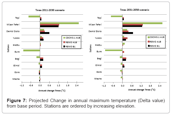
Figure 7: Projected Change in annual maximum temperature (Delta value) from base period. Stations are ordered by increasing elevation.
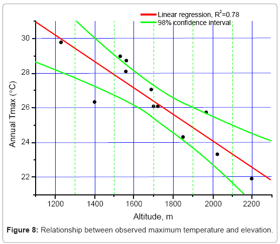
Figure 8: Relationship between observed maximum temperature and elevation.
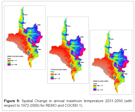
Figure 9: Spatial Change in annual maximum temperature 2031-2050 (with respect to 1972-2000) for REMO and CGCM3.1).
Other studies in Ethiopia and the Nile basin in particular using CGCM show similar pattern to this work. Hulme et al. (2001) found mean temperatures for CGCM1 B1 scenario increasing to 0.8°C in 2020s and 1.2°C in 2050s in Ethiopia. Mc Sweeney et al. [30] also shows an increase in mean temperatures in Ethiopia by 0.9°C to 1.6°C for 2030s and 1.7°C to 2.9°C for 2060s A1B scenario, and 0.5°C to 1.1°C by 2030s and 1.1°C to 1.8°C for 2060s for B1 scenario. Elshamy et al. [4] also reported an average increase in temperature over Nile basin is 2°C-4.3° C by year 2050 from 7 different CGMs. Conway (2005) also indicates that, with respect to the future climate in the Nile basin, there is high confidence that the temperature will increase. Nevertheless, this work focuses only on the catchment level and uses REMO highresolution regional model with 0.5° Lat/ Lon in addition to CGCM which were not tested in the region, further application of SDSM was the first time in the basin.
Elevation is linearly regressed and correlated with annual maximum temperature and the relationship is shown in Figure 8. In almost all cases, the actual values are confined within one standard deviation of the regression line. Elevation is negatively and highly significantly correlated (R2=0.78) for maximum temperature. This implies that elevation has a dominant role in the modification of the annual minimum and maximum temperature fields. After multiple linear regression we also found that there is higher negative correlation (R2=0.91) between altitude, latitude and annual maximum temperature, and this implies that altitude and latitude has a dominant role in the modification of annual temperature, and this relation is used to create a raster map (Figure 9) which shows temperature changes over the basin based on a 90 meter DEM. From the analysis it was possible to see temperature changes across the basin spatially. Figure 9 shows higher temperature changes likely in the lowland (western basin) and minimum change in highland (East basin).
Minimum temperature: As regards to minimum temperature the future scenario does not show similar trends across the basin. Decreasing annual trend is likely for minimum temperature in all stations except Mettu, Mezan Teferi, Gore and Bure with the range of -1.89°C to -0.1°C for both REMO A1B and B1 scenario, Whereas Stations Mettu, Mezan Teferi, Gore and Bure projected to +0.1°C to +0.82°C for REMO in the time horizon, here the projection shows that minimum temperatures have increased slightly faster than maximum temperatures for these four stations. Even though variability is observed among the stations for CGCM3.1 A1B,generally increasing annual trend is expected in the range of +0.06°C to +1.55°C for all stations except Dembi Dollo and Tepi which shows decreasing trend like REMO as shown in Figure 10.
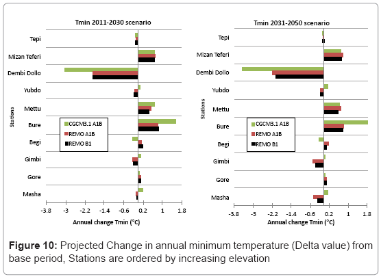
Figure 10: Projected Change in annual minimum temperature (Delta value) from base period, Stations are ordered by increasing elevation
Furthermore to elaborate the influence of elevation on average annual temperature within the upper Baro-Akobo river basin, a regression analysis was done. The outputs of the regression analysis are depicted in Figure 11. The figure shows a linear relationship plot between mean minimum temperature and elevation. The actual values in this plot are contained within one standard deviation of the regression line. The middle line (red) is the regression line; the two external lines (green) are lines of the 98% confidence interval. To quantify the relationship between the annual minimum temperature and the elevation, a regression analysis is performed. The analysis shows that the linear relationships between these two physical quantities are negative and significant (R2=0.40).
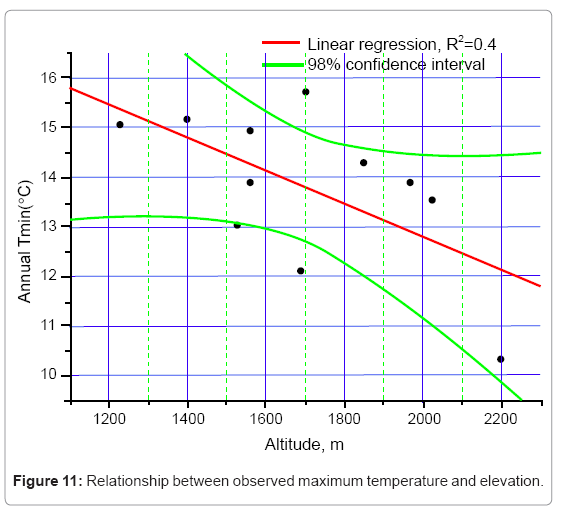
Figure 11: Relationship between observed maximum temperature and elevation.
Precipitation: In case of annual rainfall trend as shown in Figure 12, it is general likely to have a change of -2% to +21% from the base period for both A1B and B1 scenario of REMO. However, theA1B scenario of CGCM3.1projected -25% to +22% changes annually over the study area in the time horizon. Yet, each station perceives a different trend. From the REMO model 10 stations show increasing annual rainfall for A1B and B1 scenario within the range of +1% to +22%and +0.5% to +21% respectively. However, stations like Bure and Mettu show a decreasing trend for both scenarios of REMO. Regarding CGCM3.1 annual rainfall is expected to have an increasing trend in the range of +0.3% to +25% for nine stations in the basin and a decreasing trend for stations like Begi and Yubdo.
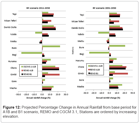
Figure 12: Projected Percentage Change in Annual Rainfall from base period for A1B and B1 scenario, REMO and CGCM 3.1, Stations are ordered by increasing elevation.
Looking of the precipitation change scenario at seasonal or monthly level has great practical importance, because in the basin activities like agriculture and water supply depend on rainfall. The basin has only one rainy season “Kiremt” begins mid of May and ends mid of October (MJJASO) for the northern part of the basin, whereas for the southern part of the basin it starts in March and ends mid of October (MAMJJASO). Kiremt’s precipitation change did not manifest a systematic increase or decrease for both REMO (A1B and B1) and CGCM3.1 (A1B) scenario. About -3% kiremt precipitation changes are expected for stations Bure, Dembi Dollo and Mettu for both REMO A1B and B1 scenario in all time horizons (Figure 13). Generally REMO shows Kiremt precipitation change in the range -22% to +25% and -21% to +13% for both A1B and B1 scenario respectively in 2011- 2050, except stations Tepi and Chora which show a +48% change. As indicated in Figure 13, CGCM3.1 A1B scenario projected Kiremt rainfall likely to change by -37% to +44% for the study area in 2011- 2050. Generally both models (REMO and CGCM3.1) shows a similar direction of change for rainy seasons in the time period (2011-2050), nevertheless higher differences are found for stations Bure, Begi and Yubdo between REMO A1B and CGCM3.1 A1B (Figure 13).
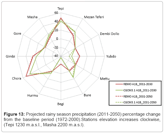
Figure 13: Projected rainy season precipitation (2011-2050) percentage change from the baseline period (1972-2000).Stations elevation increases clockwise, (Tepi 1230 m.a.s.l., Masha 2200 m.a.s.l).
Monthly rainfall also shows a similar trend to that of annual or rainy season precipitation which lack systematic trend. There is variability within the stations in the monthly rainfall but this variation in the annual rainfall is less because it considers the precipitation change in the dry season also which has no significance since the driest months contribute to less than 1% of the annual rainfall in the study area. Therefore, it is wise to see the change in the time horizon at a monthly or seasonal time scale.
Different studies in the Nile basin and the country in general figureout that future rainfall change does not verify systematic decreasing or increasing [4,8,9]. This study also confirms overall annual future rainfall trend in the basin is increasing and consistent with IPCC 4 projection. However, the models (REMO and CGCM3.1) agreed on direction of change except some stations regardless of the magnitude. Conway [8] pointed out that there are large inter-model differences of rainfall change over Ethiopia. Humle et al. [31] also found that mean annual rainfall in Ethiopia for the 2050s is expected to change in between the range of -10% to 25% considering 7 GCM models. Figure 14 shows annual trends of percentage rainfall changes (2011-2050) considering 20 runs of uncertainty ensembles for A1B scenarios of REMO and CGCM3.1.
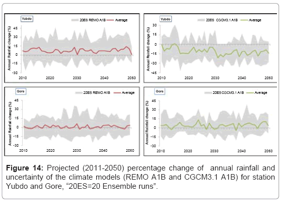
Figure 14: Projected (2011-2050) percentage change of annual rainfall and uncertainty of the climate models (REMO A1B and CGCM3.1 A1B) for station Yubdo and Gore, “20ES=20 Ensemble runs”.
Conclusion
This study analysed the output of regional (REMO) and global (CGCM3.1) climate change simulation. Downscaled precipitation and temperature were assessed over the Baro-Akobo basin for baseline climatology (1972-2000) and for the 2011-2050 aggregated in 20 years period. It appears that REMO is able to reproduce the precipitation and temperature observed over the basin. In this study maximum effort was made to assess rainfall and temperature change projections, and our main conclusions can be summarized as follows:
• Output shows SDSM smooth out the bias of REMO and CGCM3.1 during downscaling, and we found that SDSM can be used as a tool for downscaling for this region.
• Both model (REMO and CGCM3.1) projections show relatively good agreement on the direction of annual rainfall change regardless of magnitude at station scale over the basin.
• Both models indicate an increasing trend in annual maximum temperature for most of the stations with noticeable seasonal variations. The change was found to be higher in drier months (Bega) and lower in rainy season (Kiremt).
• Important finding of this study is that temperature change is inversely correlated with altitude.
• Rainfall changes show considerable uncertainty over the basin during rainy season (-20% to +50%).
• In general, SDSM approximate the observed climate data corresponding to the base period reasonably well, however the analysis of the downscaled future climate data from REMO and CGCM3.1 does not lead to identical conclusions.
Studies show that different GCMs have different projections and subject to uncertainty with respect to the many modeling issues involved. Therefore further studies in the basin have to be done considering additional climate models and exploring the relationships between climate and land use change in the basin, especially as it related to the new huge commercial farm projects. The methods described in this paper could be used to provide an indication to the likely impact of climate change in Baro-Akobo basin.
Acknowledgments
Daily meteorological data in the basin were kindly provided by Ethiopian National Meteorological Services Agency. The authors would like to acknowledge the Data Access Integration (DAI, see http://quebec.ccsn.ca/DAI/) Team for providing the data and technical support. The DAI data download gateway is made possible through collaboration among the Global Environmental and Climate Change Centre (GEC3), the Adaptation and Impacts Research Division (AIRD) of Environment Canada, and the Drought Research Initiative (DRI). The Ouranos Consortium (in Québec) also provides IT support to the DAI team. This work has been jointly supported by Federal Democratic Republic of Ethiopia via ECBP (Engineering Capacity Building Programme) and the German Academic Exchange Service (DAAD) through three years scholarship.
2 Source: http://loki.ouranos.ca/DAI/CGCM3_predictors-e.html
References
- Solomon S, Qin D, Manning M, Chen Z, Marquis M, et al. (2007) Contribution of Working Group I to the Fourth Assessment Report of the Intergovernmental Panel on Climate Change, 2007. Cambridge University Press, Cambridge, United Kingdom and New York, NY, USA.
- Solomon S, Qin D, Manning M, Chen Z, Marquis M, et al. (2007) Summary for Policymakers. In: Climate Change 2007: The Physical Science Basis. Contribution of Working Group I to the Fourth Assessment Report of the Intergovernmental Panel on Climate Change. Cambridge University Press, Cambridge, UK and NY, USA.
- Di Baldassarre G, Elshamy M, van Griensven A, Soliman E, Kigobe M, et al. (2011) Future hydrology and climate in the River Nile basin: a review. Hydrol Sci J 2:199-211.
- Elshamy ME, Seierstad IA, Sorteberg A (2009) Impacts of climate change on Blue Nile flows using bias-corrected GCM scenarios: Hydrol Earth Syst Sci 13: 551-565.
- Wing H, Cheung A, Gabriel BS , Singh A (2008) Trends and spatial distribution of annual and seasonal rainfall in Ethiopia. Int J Climatol 13: 1723-1734.
- Taye MT, Ntereka V, Ogiramoi NP, Willems P (2011) Assessment of climate change impact on hydrological extremes in two source regions of the Nile Basin. Hydrol Earth Syst Sci 15: 209-222.
- Beyene T, Lettenmaier DP, Kabat P (2010) Hydrological impact of climate change on the Nile River Basin; implication of the 2007 IPCC scenarios. Climate change 100: 433-461.
- Conway D (2005) From head water tributaries to international river: Observing and adapting to climate variability and change in the Nile basin. Global Environmental Change 15: 99-114.
- Yimer G, Andreja J, van Griensven A (2009) Hydrological Response of a Catchments to Climate Change in Upper Beles River Basin, Upper Blue Nile, Ethiopia, Nile basin Water Engineering Scientific Magazine 2: 49-59.
- Bardossy A (2000) Stochastic downscaling methods to assess the hydrological impacts of climate change on river basin hydrology. Climate Research Unit, UEA: Norwich, UK, KNMI: The Netherlands 18-34.
- Dibike YB, Gachon P, St-Hilaire A, Ouarda TBMJ, Nguyen Van T-V (2008) Uncertainty analysis of statistically downscaled temperature and precipitation regimes in Northern Canada. Theoretical and Applied Climatology 91: 149-170.
- Dibike YB, Coulibaly P (2005) Hydrological impact of climate change in the Saguenay watershed: comparison of downscaling methods and hydrologic models. Journal of Hydrology 307: 145-163.
- Xu CY, Widen E, Halldin S (2005) Modelling Hydrological Consequence of Climate Change−Progress and Challenges. Advances in Atmospheric sciences 22: 789-797
- Wilby RL, Dawson CW (2012) The Statistical Downscaling Model: insights from one decade of application. International Journal of Climatology.
- Anandhi A, Srinivas VV, Nanjundiah RS, Kumar DN (2008) Downscaling precipitation to river basin in India for IPCC SRES scenarios using support vector machine. International Journal of Climatology 28: 401-420.
- Wilby RL, Dawson CW, Barrow EM (2002) SDSM-a decision support tool for the assessment of regional climate change impacts. Environmental Modelling & software 17: 147-159.
- Wilby R, Charles SP, Zorita E, Timbal B, Whetton P, et al. (2004) Guidelines for use of climate scenarios developed from statistical downscaling methods. In: Intergovernmental Panel on Climate Change.
- Wilby RL, Dawson CW (2007) SDSM 4.2 — A decision support tool for the assessment of regional climate change impacts, User Manual. Department of Geography, Lancaster University, UK.
- Wilby RL, Wigley TML (2000) Precipitation predictors for Downscaling: Observed and General Circulation model relationships, Int J Climatol 20: 641-661.
- Khan MS, Coulibay P, Dibike Y (2006) Uncertainty analysis of statistical downscaling methods. Journal of Hydrology 316: 357-382.
- Jacob D (2001) A note to the simulation of the annual and inter-annual variability of the water budget over the Baltic Sea drainage basin. Meteorology and Atmospheric Physics 77: 61-73.
- Paeth H (2005) The climate of tropical and northern Africa – A statistical-dynamical analysis of the key factors in climate variability and the role of human activity in future climate change. Asgard-Verlag: St. Augustin Hippe, Rheinische Friedrich-Wilhelms-Universita¨t Bonn, Germany.
- Paeth H, Thamm HP (2007) Regional modelling of future African climate north of 15°S including greenhouse warming and land degradation. Climatic Change 83: 401-427.
- McFarlane NA, Scinocca JF, Lazare M, Harvey R, Verseghy D, et al. (2005) The CCCma third generation atmospheric general circulation model. CCCMA Internal Rep 25.
- Scinocca JF, McFarlane NA, Lazare M, Li J, Plummer D (2008) The CCCma third generation AGCM and its extension into the middle atmosphere. Atmos Chem and Phys 8: 7055-7074.
- DIA CGCM3 Predictors (2008) Set of Predictor Variables Derived from CGCM3 T47 and NCEP/NCAR Reanalysis, version 1.1, Monterial, QC, Canada.
- NMSA (1996) Climate and agro climatic resources of Ethiopia. NMSA (National Meteorological Service Agency) Meteorological Research Report Series 1.
- Araujo MB, New M (2006) Ensemble forecasting of species distributions. TRENDS in Ecology and Evolution. 22: 1.
- Rössler O, Diekkrüger B, Löffler J (2012) Potential drought stress in a Swiss mountain catchment—Ensemble forecasting of high mountain soil moisture reveals a drastic decrease, despite major uncertainties. Water Resour Res 48: W04521.
- McSweeney C, New M, LizcanoG, Lu X (2010) The UNDP Climate Change Country Profiles: improving the accessibility of observed and projected climate information for studies of climate change in developing countries. Bulletin of the American Meteorological Society 91: 157-166.
- Hulme M, Doherty R, Ngara T, New M, Lister D (2001) African climate change: 1900-2100, climate Research 17: 145-168.
Citation: Kebede A, Diekkrüger B, Moges SA (2013) An Assessment of Temperature and Precipitation Change Projections using a Regional and a Global Climate Model for the Baro-Akobo Basin, Nile Basin, Ethiopia. J Earth Sci Climate Change 4: 133. DOI: 10.4172/2157-7617.1000133
Copyright: ©2013 Kebede A, et al. This is an open-access article distributed under the terms of the Creative Commons Attribution License, which permits unrestricted use, distribution, and reproduction in any medium, provided the original author and source are credited.
Select your language of interest to view the total content in your interested language
Share This Article
Recommended Journals
Open Access Journals
Article Tools
Article Usage
- Total views: 19820
- [From(publication date): 3-2013 - Nov 29, 2025]
- Breakdown by view type
- HTML page views: 14231
- PDF downloads: 5589