Analytical Solution of the Groundwater Flow Equation obtained via Homotopy Decomposition Method

Groundwater models describe the groundwater flow and transport processes using mathematical equations based on certain simplifying assumptions. These assumptions typically involve the direction of flow, geometry of the aquifer, the heterogeneity or anisotropy of sediments or bedrock within the aquifer, the contaminant transport mechanisms and chemical reactions. Because of the simplifying assumptions embedded in the mathematical equations and the many uncertainties in the values of data required by the model, a model must be viewed as an approximation and not an exact duplication of field conditions. Groundwater models, however, even as approximations are a useful investigation tool that groundwater hydrologists may use for a number of applications. The equation under investigation here is given below as:

                                                                (1.1)

The equation (1.1) is subjected to the following initial and boundary conditions

.

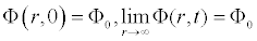
where:

S : is the specific storativity

T : the transmissivity of the aquifer

?(x,t): the piezometric head

∂_t : the time derivative

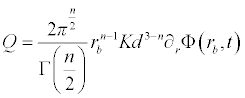
Q: is the constant discharge rate of the borehole

Several Authors have proposed a solution to this model see for example [1-6]. The purpose of this paper is to proposed an analytical solution using homotopy perturbation method.

To illustrate the basic idea of this method we consider a general nonlinear non-homogeneous partial differential equation with initial conditions of the following form

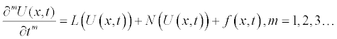                        (2.1)   

Subject to the initial condition

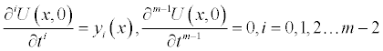
m is the order of the derivative

Where, f is a known function, N is the general nonlinear differential operator and L represents a linear differential operator and m is the order of the derivative. The method first step here is to apply the inverse operator of on both sides of equation (2.1) to obtain

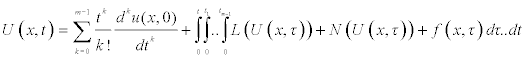          (2.2)

The multi-integral in Eq (2.1) can be transformed to [7].

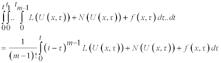
So that equation (1.2) can be reformulated as

             (2.3)

Using the Homotopy scheme the solution of the above integral equation is given in series form as:

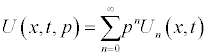                                                                                          (2.4)

and the nonlinear term can be decomposed as

Where pε[0, 1] is an embedding parameter. H_n(U) is the He’s polynomials [8-15] that can be generated by

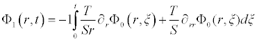
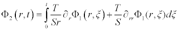
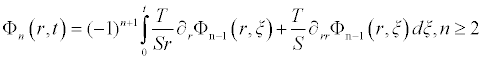
The homotopy decomposition method is obtained by the graceful coupling of decomposition method with He’s polynomials and is given by

with

                                                                                                     (2.5)

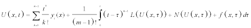
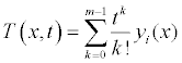
Comparing the terms of same powers of p, give solutions of various orders. The initial guess of the approximation is T(x,t).

Following the discussion presented above, we apply the inverse operator of ∂_t on both sides of Eq (1.1) to obtain

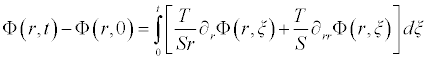                                   (3.1)

and the homotopy decomposition method is given here as:         

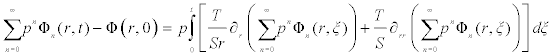     (3.2)

Comparing the terms of same powers of p give solutions of various orders we obtain the following set of equation

. . .

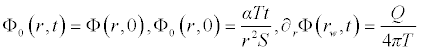
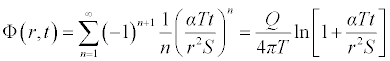
It is worth noting that if the zeroth component Φ₀ (r,t) is defined, then the remaining components n ≥ 1, can be completely determined such that each term is determined by using the previous terms, and the series solutions are thus entirely determined. Finally, the solution Φ (r,t) is approximated, for example choosing, 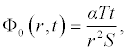the following solutions are obtained

. . .

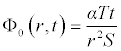
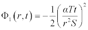
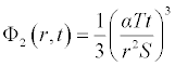
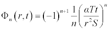
Therefore, applying the boundary condition, the approximated solutions can be given as:

Now choosing α=2.20 and converting the natural ln to Log, we obtained the following

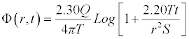                                                                           (3.3)

Several solutions of the above partial differential equation have been recently proposed; see for example Theis [4], Cooper Jacob. On one hand Theis solution was an exact solution to the partial differential equation and this solution is given below as:

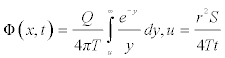                                                                                      (4.1)

However, for practical purpose this solution is very difficult to implement. On the other hand Cooper Jacob proposed an approximate solution of the partial differential equation for a latter time and this solution is given below as [5]

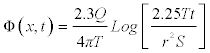                                                                                         (4.2)

The Cooper Jacob is the most used in groundwater studies because it is very easy to handle because at the time the solution was proposed, it was very easy to manipulate with the Log paper than the Theis solution (Theis solution involves exponential integral), but now day many computational software are available to handle Theis without Log paper. Nevertheless the Cooper Jacob solution has limitations, because the Cooper and Jacob solution is a large time approximation of the Theis non-equilibrium method. The approximation involves truncations of an infinite series expansion for the Theis well function that is valid when the variable: is small enough which the case in groundwater study is not always. To assess the accuracy of the method, compare the solution obtained via the homotopy decomposition method with the existing solutions including Theis and Cooper Jacob.

                                                                                  (4.3)

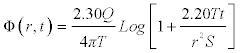
The following Figures 1-4 shows the graphical representation of the solutions for different values of theoretical properties of the aquifer. The red line is the graphical representation of the solution proposed by Cooper Jacob, the green line is the graphical representation of the solution proposed by the author and the blue line is the graphical representation of the solution proposed by Theis.

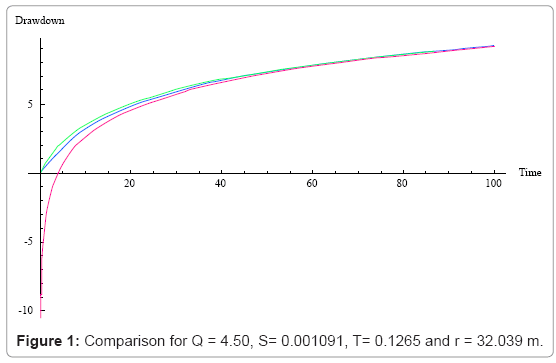
Figure 1: Comparison for Q = 4.50, S= 0.001091, T= 0.1265 and r = 32.039 m.

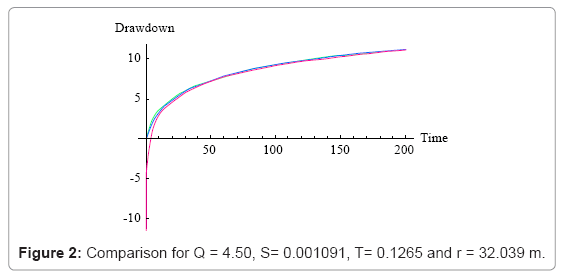
Figure 2: Comparison for Q = 4.50, S= 0.001091, T= 0.1265 and r = 32.039 m.

Figure 3: Comparison for Q = 4.50, S= 0.001091, T= 0.1265 and r = 20 m.

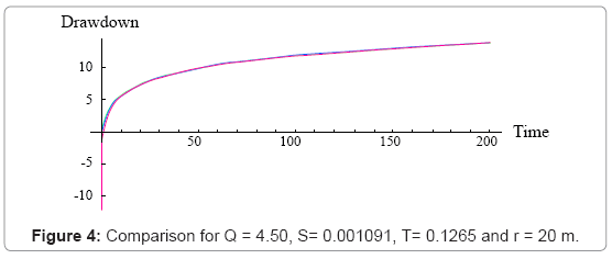
Figure 4: Comparison for Q = 4.50, S= 0.001091, T= 0.1265 and r = 20 m.

The above figure shows that for large distance from the observation borehole, the Cooper Jacob is not valid for Theis equation, meaning fitting a set of experimental data with this solution under this condition will lead to a wrong estimation of aquifer parameters under investigation, or in the same condition one can see that the solution proposed approximate successfully Theis solution.

In order to examine the validation of this solution, the above asymptotic solution is compared with 2 sets of experimental see Figures 5 and 6.

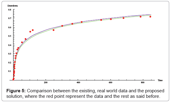
Figure 5: Comparison between the existing, real world data and the proposed solution, where the red point represent the data and the rest as said before.

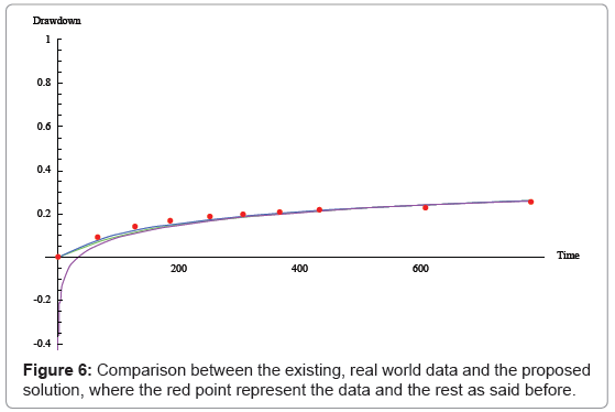
Figure 6: Comparison between the existing, real world data and the proposed solution, where the red point represent the data and the rest as said before.

The above shows the comparison between experimental data from a pumping test conducted in the polder ‘Oude Korendijk’, south of Rotterdam [15] with Cooper Jacob, Theis and the proposed solutions. Here the transmissivity was determined as T =360 m³ per day, the storativity S = 0.179 and for a constant discharge rate of Q = 9.12 l/s at a distance of r = 90 m.

The above shows the comparison between experimental data from a pumping test conducted in the p older ‘Oude Korendijk’, south of Rotterdam [16] with Cooper Jacob, Theis and the proposed solutions. Here the transmissivity was determined as T =360 m³ per day, the storativity S = 0.9 and for a constant discharge rate of Q = 9.12 l/s at a distance of r = 215 m.

In this paper, we make use of the homotopy decomposition recently proposed by Abdon Atangana to solve the groundwater flow equation. The solution obtained via the method was compared to the existing solutions including Theis and Cooper Jacob. To test the validity of the solution we compare it with two set of experimental data from real world situation. The first is from a pumping test conducted in the polder ‘Oude Korendijk’, south of Rotterdam, the Netherlands [16]. For this last set, the well screen was installed over the whole thickness of the aquifer, and piezometers were placed at distances of 30, 90, and 2 15 m from the well, and at different depths. The well was pumped at a constant discharge of 9.12 I/s for nearly 14 hours. The graphical representations of the comparison revealed a good agreement of experimental data with the proposed solution.

The authors would like to thank the referees for their comments and discussions. This work was partially supported by the National Research Fund (NRF) of South Africa.

References

- Barker JA (1988) A generalised radial flow model for hydraulic tests in fractured rock. Water Resour Res 24: 1796-1804.
- Atangana A (2012) Numerical solution of space-time fractional derivative of groundwater flow equation. International conference of algebra and applied analysis, June 20-24, Istanbul.
- Botha JF, Cloot AH (2006) A generalized groundwater flow equation using the concept of non-integer order. Water SA 32: 1.
- Theis CV (1935) The relation between the lowering of the piezometric surface and the rate and duration of discharge of a well using groundwater storage. Trans Amer Geophys Union 16: 519-524.
- Jacob CE, Lohman SW (1952) Non-steady flow to a well of constant drawdown in an extensive aquifer. Trans Amer Geophys Union 33: 559-569
- Bear J (1972) Dynamics of Fluids in Porous Media. American ElseÂvier Environmental Science Series, Elsevier, New York, USA.
- Podlubny I (2002) Geometric and physical interpretation of fractional integration and fractional differentiation. Fract Calculus Appl Anal 5: 367-386
- He JH (2002) Modified Lindstedt–Poincare methods for some strongly non-linear oscillations: Part I: expansion of a constant. Int J Non-linear Mech 37: 309-314.
- He JH (1999) Homotopy perturbation technique. Comput Methods Appl Mech Engrg 178: 257-262.
- He JH (2000) A coupling method of homotopy technique and perturbation technique for nonlinear problems. Int J Non-Linear Mech 35: 37-43.
- He JH (2003) A simple perturbation approach to Blasius equation. Appl Math Comput 140: 217-222.
- He JH (2005) Application of homotopy perturbation method to nonlinear wave equations. Chaos, Solitons & Fractals 26: 695-700.
- He JH (2005) Homotopy perturbation method for bifurcation of nonlinear problems. Int J Nonlin Sci Numer Simul 6: 207-208.
- He JH (2006) Homotopy perturbation method for solving boundary value problems. Phys Lett A 350: 87-88.
- He JH (2006) Non-perturbative Methods for Strongly Non-linear Problems. Germany: Die Deutsche bibliothek.
- Wit KE (1963) The hydraulic characteristics of the Oude Korendijk polder, calculated from pumping test data and laboratory measurements of core samples (in Dutch). Inst L and and Water Manag Res, Wageningen, Report No. 190,24.
Citation: Atangana A, Botha JF (2012) Analytical Solution of the Groundwater Flow Equation obtained via Homotopy Decomposition Method. J Earth Sci Climate Change 3: 115. DOI: 10.4172/2157-7617.1000115
Copyright: ©2012 Atangana A, et al. This is an open-access article distributed under the terms of the Creative Commons Attribution License, which permits unrestricted use, distribution, and reproduction in any medium, provided the original author and source are credited.
Select your language of interest to view the total content in your interested language
Share This Article
Recommended Journals
Open Access Journals
Article Tools
Article Usage
- Total views: 17276
- [From(publication date): 7-2012 - Dec 20, 2025]
- Breakdown by view type
- HTML page views: 12247
- PDF downloads: 5029