Climate Change Impacts on the Ou é m é River, Benin, West Africa
Received: 04-Sep-2013 / Accepted Date: 22-Sep-2013 / Published Date: 30-Sep-2013 DOI: 10.4172/2157-7617.1000161
Abstract
The present study identifies the future impacts of climate change on the flows of the Ouémé River in Bonou, for the 2035-2064 and 2070-2099 periods. For this identification, a set of 65 climate projections from 24 climate models, based on three greenhouse gas emissions scenarios (A2, B1 and A1B) was used. Hydrologic simulations were carried out with a lumped conceptual hydrology model. The results obtained from this study show that daily temperatures in the Ouémé catchment over the reference period (1971-2000) will raise by up to 5°C during the 2070-2099 horizon. For their part, mean daily precipitation projections are much more uncertain. However, what is clear is that mean monthly flows will see a drop potentially as high as 30% during the rainy season, and 20% during the dry season. Similarly, mean seasonal and annual flows will drop by as much as 8 to 10% and 3 to 5%, respectively. This drop will also affect maximum annual flows at a proportion of approximately 3% in the 2035-2064 period and of 5% between 2070 and 2099. This study also showed that we will be seeing changes in extreme flows. These changes will be characterized by a slight drop in quantiles for return periods of less than 10 years, and a potential increase of up to 100 m3/s (an increase of approximately 6%) for quantiles of the return period of 100 years covering the 2070-2099 horizon. These changes have impacts on the economic activities and on the water resource availability in the catchment.
Keywords: Climate change; Hydrology model; Impacts; Flows; Water availability
11167Introduction
Global climate change has a significant influence on regional water resources [1-3]. Africa is one of the continents that are most vulnerable to the effects of climate change. It’s vulnerability particularly that of subsaharan countries is compounded by its low adaptation capacity [4]. Fluctuations due to climate change have an impact on catchments [5,6]. They can result in long periods of drought or of excess precipitations; they can have long-lasting impacts on the hydrological cycle, and can significantly affect the quantity of available water resources [7]. That was the case in West Africa, which experienced a major drought from the 70s to the 90s [8], which resulted in a 20 to 30% drop in annual precipitations [9,10].
In Benin, and particularly in the Ouémé catchment, this decrease in rainfall led to a change in the hydrology regime and in a drop in economic activity along the Ouémé River [8]. This is the biggest river in the Republic of Benin, and drains parts of the north, centre and southern areas of the country [11]. Fishing along this river accounts for approximately 73% of Benin's fish industry [12]. Furthermore, the water volumes extracted from the river are used for agriculture (64%), which is practised by 61.1% of the population in the entire catchment, for domestic purposes (30%) and for livestock farming (6%) [12,13].
Given the important role played by this river, it is therefore essential to know the future potential impacts climate change will have on its hydrology regime, so as to be able to anticipate adequate strategies to implement in order to prevent the adverse effects that could result from doing nothing.
This work therefore aims to identify the impacts over the 2035- 2064 and 2070-2099 horizons. This study used the outputs of 24 climate models from 24 international modelling centres currently contributing to the international dataset.
Study Area
The geographic area covered in this study is the Ouémé catchment. With a surface area of approximately 50,000 km2, the Ouémé catchment is characterized by two climates: a subequatorial climate to the south (up to the latitude of Bohicon) and a Sudanian climate to the north. One part of the Ouémé catchment is located on the Dahomey side (Ouémé Supérieur) and the other part is situated on the sedimentary rock formations of the coastal basin (Ouémé Inférieur). Mean daily precipitation in the Ouémé catchment over the last 5 decades is 3.2 mm, and mean annual minimum and maximum daily temperatures are 21.6°C and 32.6°C, respectively. The Ouémé catchment is drained by the biggest river in Benin, the Ouémé River. The Ouémé River (situated between 6°30’ and 10° North latitude), is 510 km long, and originates at the Atacora chain in North Benin, and flows all the way to the south, where it feeds the Nokoué lake lagoon system and the Porto-Novo lagoon. The mean annual daily flow of the Ouémé River in Bonou for the last 5 decades is 170 m3/s (Figure 1).
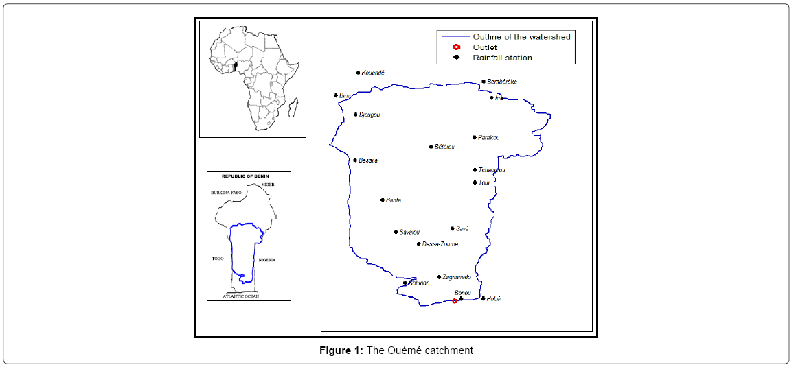
Figure 1: The Ouémé catchment
Materials And Methods
Materials
Data used: Two types of data were used: observation data for the reference period (1971-2000) obtained from eighteen (18) weather stations built on the Ouémé catchment and in the surrounding areas, and the outputs of 24 climate models for the reference period and for two future periods: 2035-2064 and 2070-2099.
Observation data consist of annual minimum and maximum daily temperatures and of daily precipitations. The geographic coordinates of the eighteen (18) weather stations used for daily precipitation data are presented in Table 1. As illustrated in the table, daily temperature data are taken from three of these stations.
| N° | Station | Coordinates | Data used | |
|---|---|---|---|---|
| North Latitude | East Longitude | |||
| 1 | Ina | 09°57’ | 02°43’ | P |
| 2 | Savé | 07°58’ | 02°25’ | P, T |
| 3 | Toui | 08°40’ | 02°36’ | P |
| 4 | Pobé | 06°55’ | 02°39’ | P |
| 5 | Birni | 09°58’ | 01°30’ | P |
| 6 | Banté | 08°24’ | 01°52’ | P |
| 7 | Bonou | 06°55’ | 02°30’ | P |
| 8 | Bassila | 09°00’ | 01°39’ | P |
| 9 | Savalou | 07°55’ | 01°58’ | P |
| 10 | Bétérou | 09°12’ | 02°15’ | P |
| 11 | Parakou | 09°21’ | 02°36’ | P, T |
| 12 | Bohicon | 07°09’ | 02°03’ | P, T |
| 13 | Djougou | 09°42’ | 01°39’ | P |
| 14 | Kouandé | 10°19’ | 01°40’ | P |
| 15 | Tchaourou | 08°51’ | 02°36’ | P |
| 16 | Bembéréké | 10°12’ | 02°39’ | P |
| 17 | Zangnanado | 07°15’ | 02°19’ | P |
| 18 | Dassa-Zoumé | 07°45’ | 02°09’ | P |
Table 1: Weather stations and data used
(Source: National Weather Service, 2012)
P=Precipitations; T=Temperatures
The outputs of the climate models used consist of monthly minimum and maximum temperatures (or of mean monthly temperatures) and of mean monthly precipitations. The climate models and their respective centres are presented in the following table (Table 2):
| N° | Climate model | Modelling centre | Scenario | Data used |
|---|---|---|---|---|
| 1 | BCM2.0 - Run 1 | Bjerknes Centre for Climate, Norway | A2, A1B and B1 | P, T |
| 2 | CGCM3T47–Mean | Canadian Centre for Climate Modelling and Analysis (CCCma), Canada | A2, A1B and B1 | P, T |
| 3 | CGCM3T63 - Run 1 | Canadian Centre for Climate Modelling and Analysis (CCCma), Canada | A2, A1B and B1 | P, T |
| 4 | CNRMCM3–Run 1 | Centre National de Recherches Metéorologiques, France | A2, A1B and B1 | P, T |
| 5 | CSIROMk3.0–Run 1 | Australia's Commonwealth Scientific and Industrial Research Organisation (CSIRO), Australia | A2, A1B and B1 | P, T |
| 6 | CSIROMk3.5–Run 1 | Australia's Commonwealth Scientific and Industrial Research Organisation (CSIRO), Australia | A2, A1B and B1 | P, T |
| 7 | ECHAM5OM–Mean | Max Planck Institute für Meteorologie, Germany | A2, A1B and B1 | P, T |
| 8 | ECHO-G–Mean | Meteorological Institute, University of Bonn Meteorological Research Institute, Germany | A2, A1B and B1 | P, T |
| 9 | FGOALS-g1.0–Mean | Institute of Atmospheric Physics, Chinese Academy of Sciences, China | A1B and B1 | P, T |
| 10 | GFDLCM2.0–Run 1 | Geophysical Fluid Dynamics Laboratory (GFDL), USA | A2, A1B and B1 | P, T |
| 11 | GFDLCM2.1–Run 1 | Geophysical Fluid Dynamics Laboratory (GFDL), USA | A2, A1B and B1 | P, T |
| 12 | GISS-AOM–Mean | Goddard Institute for Space Studies (GISS), USA | A1B and B1 | P, T |
| 13 | GISSE-H–Mean | Goddard Institute for Space Studies (GISS), USA | A1B | P, T |
| 14 | GISSE-R–Run 1 | Goddard Institute for Space Studies (GISS), USA | A2, A1B and B1 | P, T |
| 15 | HADCM3–Run 1 | UK Meteorological Office, United Kingdom | A2, A1B and B1 | P, T |
| 16 | HADGEM1–Run 1 | UK Meteorological Office, United Kingdom | A2 and A1B | P, T |
| 17 | INGV-SXG–Run 1 | National Institute of Geophysics and Volcanology, Italy | A2 and A1B | P, T |
| 18 | INMCM3.0–Run 1 | Institute for Numerical Mathematics, Russia | A2, A1B and B1 | P, T |
| 19 | IPSLCM4–Run 1 | Institute Pierre Simon Laplace, France | A2, A1B and B1 | P, T |
| 20 | MIROC3.2 medres–Mean | National Institute for Environmental Studies, Japan | A2, A1B and B1 | P, T |
| 21 | MIROC3.2 hires–Run 1 | National Institute for Environmental Studies, Japan | A1B and B1 | P, T |
| 22 | MRI CGCM2.3.2a–Mean | Meteorological Research Institute, Japan Meteorological Agency, Japan | A2, A1B and B1 | P, T |
| 23 | NCARCCSM3–Mean | National Center for Atmospheric Research (NCAR), USA | A2, A1B and B1 | P, T |
| 24 | NCARPCM - Mean | National Center for Atmospheric Research (NCAR), USA | A2, A1B and B1 | P, T |
Table 2: Climate models and modelling centres
(Source: Environment Canada: http://www.cccsn.ec.gc.ca/?page=dd-gcm)
P=Precipitations; T=Temperatures
Hydrology model and optimization algorithm: The hydrology model used for this study is the HMETS (Hydrology Model-ÉTS) model. It is a lumped 21-parameter conceptual model developed at the école de Technologie Supérieure (ÉTS) [14]. HMETS simulates the main hydrological processes of evapotranspiration (one parameter), snow accumulation and disappearance (ten parameters), horizontal (four parameters) and vertical transfers (six parameters). In this study, the snow module was not used, and HMETS reverted to a 11-parameters model. The HMETS code, including the automatic calibration module is freely available on the Mathworks file exchange site. The use of a global hydrology model for a watershed of this size may not be optimal, and as such, a distributed hydrology model was first considered. However, in the end, the lack of spatialized data in this region of Africa made us opt for the lumped model. As it turned out (details further below), the lumped model did a good job of modelling streamflows on the Ouémé River.
HMETS calibration in the Ouémé catchment was carried out using the (Covariance Matrix Adaptation Evolution Strategy) optimization algorithm [15,16]. It is a robust evolutionary algorithm based on the maximum likelihood principle. It is renowned for its capacity to effectively identify global optima [17].
Methodology
Data processing: Because HMETS is a lumped model; input data were averaged for the entire catchment beforehand. The Thiessen polygons method was used to average observation data. Since the climate model outputs were produced on grids, for each climate model, the data for the four (04) grid points closest to the centre of the catchment were chosen and averaged. Next, these data were averaged over the entire catchment, using the Inverse Distance Weighted (IDW) method for the catchment centroid.
Model calibration: The objective function used to calibrate the HMETS model was the Nash-Sutcliffe metric, which is commonly used in hydrology:
 (1)
(1)
where:
Qobs=observed flow
Qavg=mean of observed flows
Qsim=simulated flow
NSE=Nash Sutcliffe efficiency criteria
The value of the Nash Sutcliffe criteria varies between 1 (perfect match between observed and modelled streamflows) and -∞. A value of 0 indicates that the model performance is equivalent to that of one using the annual mean flow as a year round estimate of stream flows. A value greater than 0.5 is generally considered adequate, while a value above 0.7 is deemed good.
Calibration followed a traditional split-sample cross-validation approach, with the exception that instead of separating the historical record into two different continuous periods, odd years were first used for calibration, with even years left out for model validation. Odd and even years were then switched to perform the cross-validation. Separating the data record into odd and even years reduces potential biases in the calibration/validation process by removing natural trends linked to the climate decadal and multidecadal natural variability. The downside of this approach is that it requires that the entire record length be used during the calibration even though only half of the record is needed to compute the objective function. Model calibration takes twice as long using this approach; however, this is not a problem for a lumped model like HMETS, which has a very rapid execution time. The parameter set with the higher Nash Sutcliffe during calibration was chosen among the two obtained from the cross-validation approach.
Scaling of outputs of climate models: Various downscaling methods are available, and were developed based on a variety of approaches: factor change approaches [18-21], bias correction approaches [22-28]. In the present study, we used a factor change approach, the socalled "deltas" or "Constant Scaling (CS)" approach. The delta method is robust, simple and is widely used in the literature. Its biggest advantage is perhaps that it only requires monthly averages of precipitation and temperature, thus permitting the use of a large number of climate model outputs. Since climate models have been identified as the main source of uncertainty in many studies [29], it is critical to include as many models as possible to adequately cover the uncertainty. More complex downscaling methods require daily outputs from climate models, which limits the number of models that can be used. The deltas method consists in determining the daily temperatures of the future period (Tadjusted, fut, day) by adjusting the daily temperatures observed during the reference period (Tobs, day), and adding up the differences between the mean monthly temperatures projected by Climate Models (CM) for future reference periods (Equation (2)) [19,21]. Adjusted daily precipitations for the future period (Padjusted, fut, day) are obtained by multiplying the daily precipitations observed during the reference period (Pobs, day) by the precipitation rate  (Equation (3)).
 (2)
(2)
 (3)
(3)
In these equations, "m" and "day" respectively designate a specific given "month" and "day".
Study of the relative evolution of future flows: Future flows for each of these two periods (2035-2064 and 2070-2099) were compared to those for the reference period (1971-2000). They are: the mean monthly flows, the mean seasonal flows, the mean annual flows, and maximum flows.
The rates of flow variations were calculated as follows:
 (4)
(4)
Where Q designates the flow.
An analysis of the rates of flow allowed us to determine future flow trends.
Frequency analysis of extreme flows: The frequency analysis was carried out on maximum annual flows. The distribution function used was the Pearson III function. The function parameters were determined using the maximum likelihood method. The confidence interval used for the computations was 95%.
Results
The results will be presented in three sections: Model calibration, Climate projections and Hydrologic impacts.
Model calibration
The following results were obtained following the HMETS calibration-validation: even-odd calibration-validation (NSE)calibration=0.829 and (NSE)validation=0.937; odd-even calibration-validation (NSE)calibration=0.949 and (NSE)validation= 0.828. The set of parameters retained was that corresponding to the even-odd calibration-validation. With this set of parameters, HMETS was used to simulate the daily flows throughout the reference period. Figure 2 below presents an extract of simulation results (for the 1991-1995 period). As can be seen, the hydrogram observed is properly simulated, proving that the HMETS model adequately simulates the flows of the Ouémé River in Bonou.
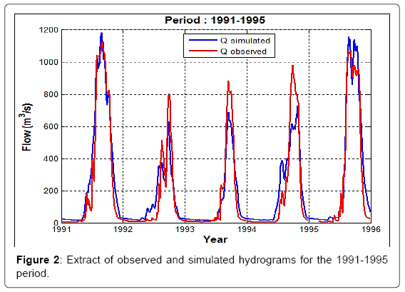
Figure 2: Extract of observed and simulated hydrograms for the 1991-1995 period.
By comparing the observed and simulated mean annual hydrograms for the reference period (1971-2000), we can see that the annual variation of mean monthly flows is adequately simulated by the HMETS hydrologic model, despite a slight overestimation of dry weather flows and an underestimation of flood flows, as illustrated in Figure 3.
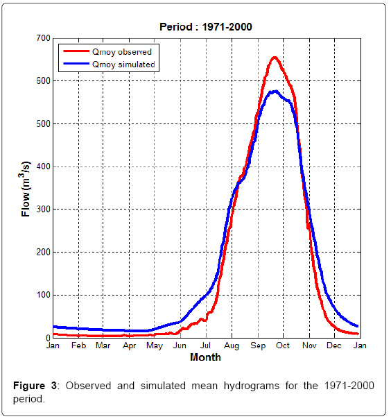
Figure 3: Observed and simulated mean hydrograms for the 1971-2000 period.
Delta factors distribution for temperatures and precipitations
The monthly distribution of temperature change factors (Figure 4) shows a general upward trend for daily temperatures for the 2035- 2064 periods. Globally, this rise should be by about 1 to 3°C. It was projected by all models for the months of April to November, in all greenhouse gas emissions scenarios considered. That was also the case for the months of December to March, with the exception of a very slight decrease (less than 1°C) forecast for December, February and March by a single model, and by 1°C to 2°C forecast for January by just two models.
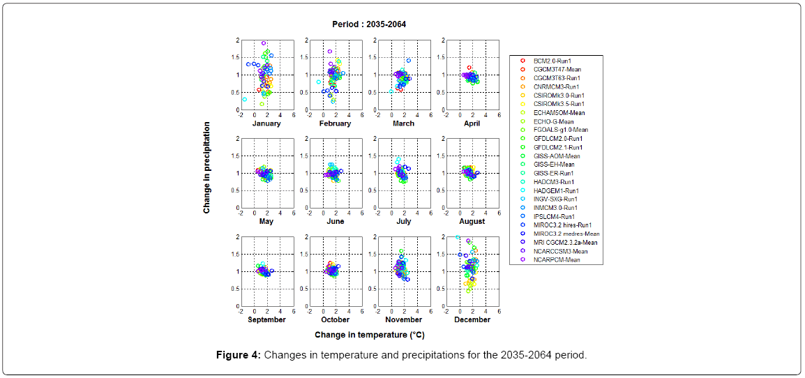
Figure 4: Changes in temperature and precipitations for the 2035-2064 period.
With regard to changes in daily precipitations for the 2035-2064 period, there is strong uncertainty with the projected trends. Indeed, for all months, we have practically as many models forecasting a decrease in daily precipitation as those forecasting an increase. However, for the months of March to May, over half the models forecast a 25% to 50% drop in daily precipitations. The greatest disparity was observed with forecasts relating to the dry season months (November-May), and particularly, for the months of December to February, which corresponds to the start of the dry season. Globally, precipitation change forecasts range between -75% and +75% in the dry season, except in December and January, respectively, where 3 and 4 models forecast a rise of over 100% (points were not represented). Regarding daily precipitation changes during the rainy season, the variations were between -25% and +50%.
For the 2070-2099 period, all the models predicted, for all greenhouse gas emissions scenarios, a rise in daily temperatures, for all months except January, where a single model (for a single SES) predicted a slight 0.5°C drop in temperatures (Figure 5). We can thus say that generally, all the models forecast a rise in daily temperatures for this future period. Unlike with the 2035-2064 period, the scope of the increase is higher (1 to 5°C).
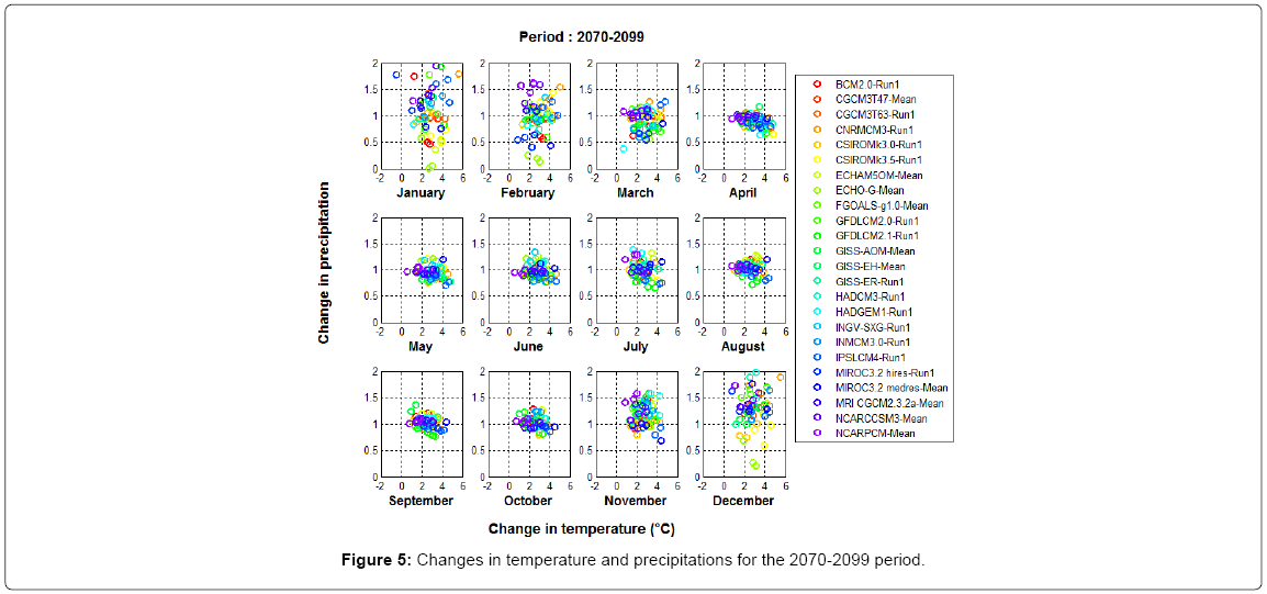
Figure 5: Changes in temperature and precipitations for the 2070-2099 period.
As with the 2035-2064 period, daily precipitation change forecasts are uncertain. Indeed, apart from the months of March and April, for which over 50% of the models forecast a drop in precipitations, and the months of November and December, for which most models indicate a rise in precipitations, practically the same number of forecasts predict a rise as do those predicting a drop. The dispersion of the forecasts is more pronounced for the months of December to February, just as in the 2035-2064 period. Similarly, for this period, projected changes in daily precipitations during the dry season were generally between -75% to +75%, except for the months of December and January, where 3 and 5 models respectively forecast a rise of over 100% (the corresponding (points were not represented). Daily precipitation changes forecast for the rainy season were between -25% and +50%.
All the previously examined forecasts indicate a rise in annual monthly temperatures, as illustrated in Figure 6. Indeed, for all the greenhouse gas emissions scenarios considered, all the climate models forecast a rise in annual mean temperatures for each of the future periods studied. For the 2035-2064 period, this rise was 0.5 to 2.5°C and rose to 4.5°C for the 2070-2099 period. That anticipates a neverending rise in temperatures throughout the catchment, which could lead to increased evapotranspiration. Forecast changes in mean annual precipitations are uncertain because, as can be seen in Figure 4, for each of the two future horizons, there is good upward and downward dispersion among the models. Nevertheless, in absolute terms, the rises forecast by some models are generally greater than the drops predicted by others.
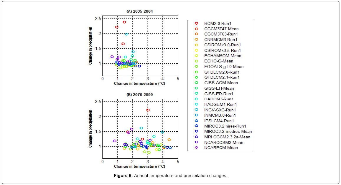
Figure 6: Annual temperature and precipitation changes.
An analysis of the relative evolution of future flows will allow a better clarification of the joint impact of temperature and precipitation changes.
Relative evolution of future flows
For future flows, we should specify that all comparisons were carried out with simulated flows for the reference period. This allows us to eliminate the intrinsic biases of the hydrologic model, and thereby represent only the real impacts of forecast climate changes.
For each of the two future periods considered, the hydrologic impact of most climate forecasts shows a drop in monthly flows (Figure 7). This drop was much more pronounced during the rainy season (June-October) than in the dry season (November to May). In the rainy season, it reached 20% (in the month of June) for the 2035-2064 horizon, and 30% (in the months of June and July) in the 2070-2099 horizon. In the dry season, it was between 5 and 20% over each of the two horizons considered. The greatest drop in the dry season was obtained in the month of May. Uncertainties regarding the results were greater for the 2070-2099 horizon than for the 2035-2064 horizon, particularly for forecasts concerning the rainy season. These results point to a projected reduction in flooding of the Ouémé River in Bonou, and to increased future low water levels.
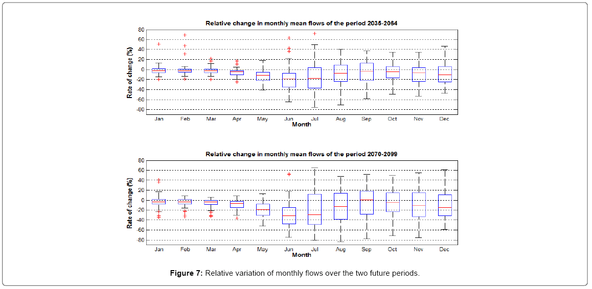
Figure 7: Relative variation of monthly flows over the two future periods.
These results were corroborated by results showing variations between mean seasonal flows, and presented in Figure 8. Indeed, for each of the two future periods, the seasonal impacts were in the form of reductions in mean seasonal flows. In the dry season, the reduction in mean seasonal flows was 5% in the 2035-2064 horizon and 8% in the 2070-2099 horizon. In the rainy season the reduction was by 10% over each of the two future periods, but with greater uncertainty for the 2070-2099 horizon.
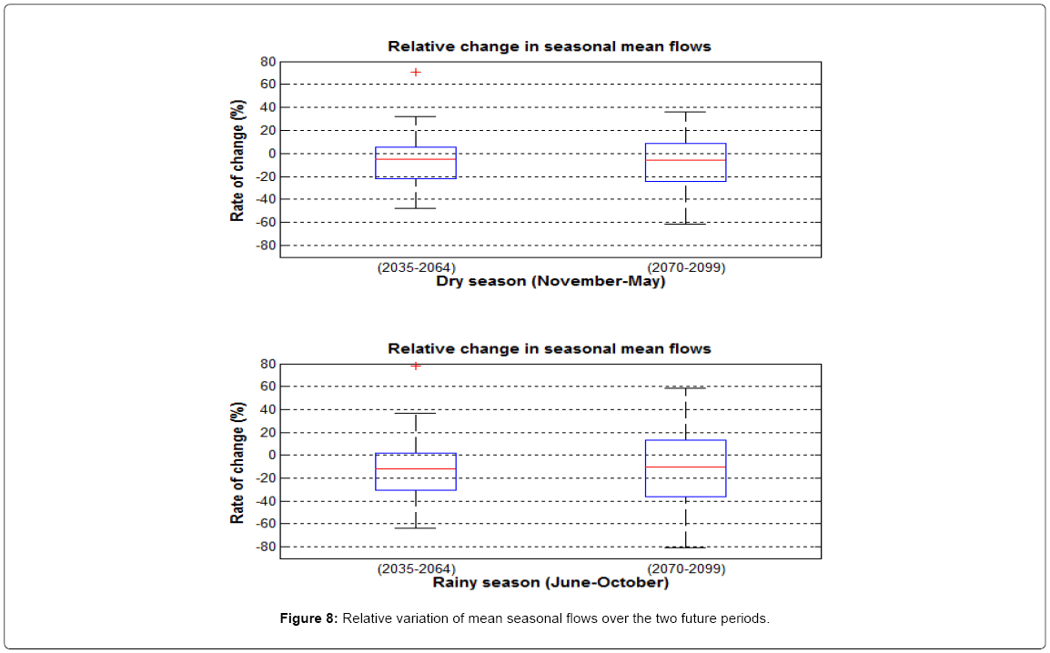
Figure 8: Relative variation of mean seasonal flows over the two future periods.
The general reduction in mean monthly flows was also manifested through a reduction in mean annual flows (Figure 9). This drop was estimated at about 8% in the 2035-2064 horizon and 10% in the 2070-2099 horizon.
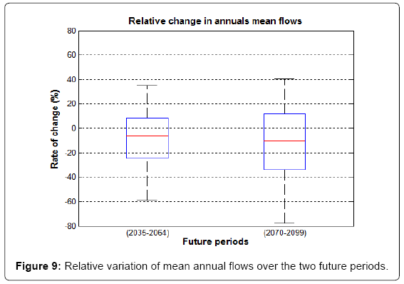
Figure 9: Relative variation of mean annual flows over the two future periods.
With regards to maximum flows, as was only to be expected given the aforementioned, the hydrologic impact of future climate forecasts will be manifested by a reduction in flows, as illustrated in Figure 10. However, the impact of these maximum flows is less pronounced than it is in the case of mean flows. In the dry season, the reduction in mean seasonal flows was 5% in the 2070-2099 horizon and 8% in the 2070- 2099 horizon.
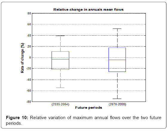
Figure 10: Relative variation of maximum annual flows over the two future periods.
Frequency analysis
Quantiles were determined for 5-, 10-, 20-, 50- and 100-year return periods. For the reference period (1971-2000), the quantiles determined from simulated flows were compared to those determined from observed flows. The results obtained are presented in Figure 11. Globally, for the 5-, 10- and 20-year return periods, the quantiles obtained from simulated flows (1005, 1211 and 1392 m3/s respectively) were practically equal to those obtained from observed flows (1029, 1213 and 1379 m3/s respectively). Beyond the 20-year return period, the quantiles determined from simulated flows were higher than those determined from observed flows. However in all cases, both values were well within the confidence interval of the estimation.
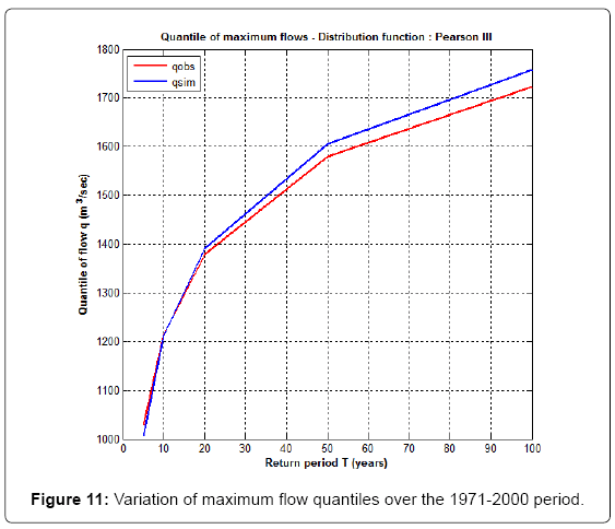
Figure 11: Variation of maximum flow quantiles over the 1971-2000 period.
As in the preceding section, the quantiles for future periods (determined from simulated annual flows) were compared to the quantiles from simulated flows over the reference period.
For the 2035-2064 future periods, the quantiles calculated for the 5- and 10-year return periods were slightly smaller than those determined over the reference period, as illustrated in Figure 12. This result was not unexpected, given the previously observed reduction in maximum annual flows. However, beyond the 10-year return period, the trend was reversed and the discrepancy between the future quantiles and those for the reference period reached 43 m3/s for the 100-year return period. The same trends observed earlier were equally observed for the 2070- 2099 period. Indeed, the future quantiles for this period were slightly lower than (or equal to) those for the reference period for the 5- and 10-year return periods (Figure 13). For the return periods greater than 10 years, the trend was also reversed. The discrepancies grew with the return period, even reaching as high as approximately 100m3/s for the 100-year return period.
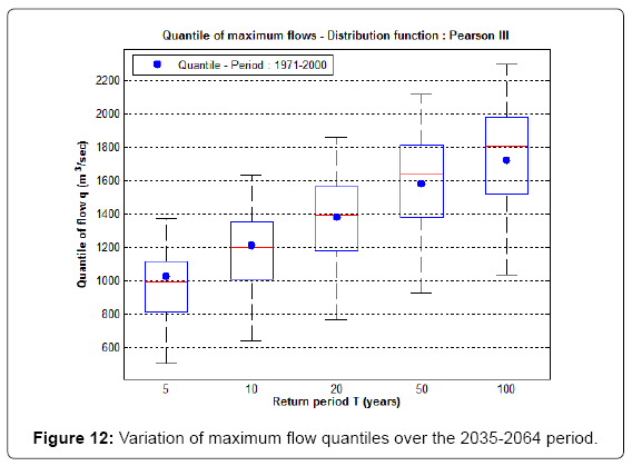
Figure 12: Variation of maximum flow quantiles over the 2035-2064 period.
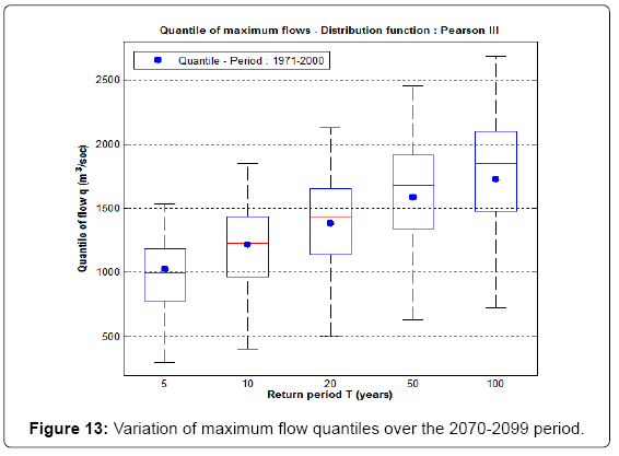
Figure 13: Variation of maximum flow quantiles over the 2070-2099 period.
Discussion
The results of the present study were obtained using a multi-climatemodel approach. According to the scientific literature, using the means and medians of several models provides the signals that best forecast climate change [30]. The models' results can vary significantly from one another because each model has its own inherent biases. However, using the means or medians of several models reduces the uncertainty associated with each individual model since, taken together, the individual models' biases would seem to level out [31,32]. The lumped results thus truly approximate historical climate data. Therefore, although lumped forecasting does not constitute a guarantee, it should be more likely to accurately simulate future climate conditions. That is why this approach was adopted.
The results' analysis showed that we should expect a steady and growing increase in daily temperatures (by between 1 and 5°C) throughout the catchment studied. Practically all climate models agree on such a trend. The probability of the Ouémé catchment experiencing future warming is thus very high. This result is consistent with those published by [33]. One of the consequences of such warming will be increased evapotranspiration, one of the components of the water balance of the catchment. If this increased evapotranspiration is not counterbalanced by increased precipitation, the result would be a reduction in flows and/or reduced groundwater replenishment. However, for precipitations, future projections have indicated (considering the projection medians) that generally, they will not be changing significantly. It is not surprising to notice reduced flows levels.
The reduction in mean monthly flows in the rainy season (by up to 30%) could somewhat alleviate the flooding as well as its scope, particularly in the city of Cotonou which is located downstream. Whatever the case, while the future extreme flows of the Ouémé River in Bonou for return periods of less than 10 years could be less intense, we must not lose sight of the fact that those for return periods of more than 10 years could be more abundant, and could thus lead to heavier and more frequent flooding.
Moreover, the reduction in mean monthly flows in the dry season (by up to 20%) could be manifested through a faster depletion of the Ouémé River.
Given all the projected reductions in flows, we could see a decline in the surface water resource in terms of available volume, with a resulting drop in the level of socio-economic activity all along the Ouémé River, such as agriculture and fishing, which are largely dependent on this resource. Furthermore, we must also anticipate a possible reduced groundwater replenishment, and thus, the decline of the water resource which largely contributes (85%), to the total volume of water used to supply the populations living in the Ouémé catchment [12].
Conclusion
This study adopted a multi-climate-model approach to determine the future impacts of climate change on the hydrologic regime of the Ouémé River in Benin. It showed that there will be a rise in mean daily temperatures, accompanied by a reduction in mean monthly flows of the river. This reduction will be observed both in the dry and in the rainy seasons, probably leading to a slowing down of economic activity and a reduction in water availability in the Ouémé catchment.
Finally, this study also showed that, compared to the reference period, extreme flows with a return period smaller than 10-year will diminish, and that for longer return periods, extreme flows are expected to be on the rise.
Acknowledgement
The authors would like to thank the reviewers for their anticipated comments and suggestions in order to improve on the quality of this manuscript.
References
- Bronstert A, Niehoff D, Bürger G (2002) Effects of climate and land use change on storm runoff generation: present knowledge and modelling capabilities. Hydrol Process 16: 509-529.
- Menzel L, Bürger G (2002) Climate change scenarios and runoff response in the Mulde catchment (Southern Elbe, Germany). J Hydrol 267: 53-64.
- Mimikou MA, Baltas E, Varanou E, Pantazis K (2000) Regional impacts of climate change on water resources quantity and quality indicators. J Hydrol 234: 95-109.
- IPCC (2001) Climate Change 2001: Impacts, Adaptation, and Vulnerability. Contribution of Working Group II to the Third Assessment Report of the Intergovernmental Panel on Climate Change, Cambridge University Press, Cambridge, UK.
- Manfreda S (2013) The Water Management in the Present Century. Hydrol Current Res 4: e105.
- Khajuria A, Ravindranath NH (2012) Climate Change in Context of Indian Agricultural Sector. J Earth Sci Clim Change 3:110.
- Afouda A, Bouchez JM, Braud I, Cazenave F, Depraetere C, et al. (2001) Variabilité climatique et variabilité hydrologique en Afrique de l’Ouest : Un système couplé. Atelier sur le Couplage des modèles atmosphériques et hydrologiques, Toulouse, France.
- Vissin E, Boko M, Perard J, Houndenou C (2003) Recherche de ruptures dans les séries pluviométriques et hydrologiques du bassin béninois du fleuve Niger (Bénin, Afrique de l'ouest). Association Internationale de Climatologie 15: 368-376.
- Lebel T, Vischel T (2005) Climat et cycle de l’eau en zone tropicale: un problème d’échelle. CR Geoscience 337: 29-38.
- L’Hôte Y, Mahé G, Some B, Triboulet JP (2002) Analysis of a Sahelian annual rainfall index from 1896 to 2000; the drought continues. Hydrolog Sci J 47: 563-572.
- Anthony EJ, Oyédé LM, Lang J (2002) Sedimentation in a fluvially infilling, barrierbound estuary on a wave-dominated, microtidal coast: the Ouémé River estuary, Benin, West Africa. Sedimentology 49: 1095-1112.
- Tossa AAY, Tonouhewa A (2009) Profil du bassin de l’Ouémé et caractérisation des sites pilotes (analyse des données), Rapport final FAO, PROJET GCP/GLO/207/ITA, Bénin.
- Yehouenou E, Pazou A, Lalèyè P, Boko M, van Gestel CAM, et al. (2006) Contamination of fish by organochlorine pesticide residues in the Ouémé River catchment in the Republic of Bénin. Environ Int 32: 594-599.
- Martel JL, Demeester K, Brissette FP (2013) HMETS-A simple and efficient hydrology model for flow forecasting, climate change studies and teaching purposes. Environmental Modelling & Software (submitted).
- Hansen N, Ostermeier A (2001) Completely Derandomized Self-Adaptation in Evolution Strategies. Evolutionary Computation 9: 159-195.
- Hansen N, Ostermeier A (1996) Adapting arbitrary normal mutation distributions in evolution strategies: The covariance matrix adaptation. Proceedings of the 1996 IEEE International Conference on Evolutionary Computation.
- Arsenault R, Poulin A, Côté P, Brissette FP (2013) A comparison of stochastic optimization algorithms in hydrological model calibration. Journal of Hydrologic Engineering. In Press.
- Chen J, Brissette F, Chaumont D, Braun M (2013) Performance and uncertainty evaluation of empirical downscaling methods in quantifying the climate change impacts on hydrology over two North American river basins. J Hydrol 479: 200-214.
- Chen J, Brissette FP, Leconte R (2011) Uncertainty of downscaling method in quantifying the impact of climate change on hydrology. J Hydrol 401: 190-202.
- Maraun D, Wetterhall F, Ireson AM, Chandler RE, Kendon EJ, et al. (2010) Precipitation downscaling under climate change: Recent developments to bridge the gap between dynamical models and the end user. Rev Geophys 48.
- Mpelasoka FS, Chiew FHS (2009) Influence of Rainfall Scenario Construction Methods on Runoff Projections. J Hydrometeor 10: 1168-1183.
- Chen J, Brissette F, Chaumont D, Braun M (2013) Finding appropriate bias correction methods in downscaling precipitation for hydrologic impact studies over North America. Water Resour Res 49: 4187-4205.
- Themeßl MJ, Gobiet A, Heinrich G (2011) Empirical-statistical downscaling and error correction of regional climate models and its impact on the climate change signal. Climatic Change 112: 449-468.
- Themeßl MJ, Gobiet A, Leuprecht A (2010) Empirical statistical downscaling and error correction of daily precipitation from regional climate models. Int J Climatol 31: 1530-1544.
- Piani C, Haerter JO, Coppola E (2010) Statistical bias correction for daily precipitation in regional climate models over Europe. Theor Appl Climatol 99: 187-192.
- Ines AVM, Hansen JW (2006) Bias correction of daily GCM rainfall for crop simulation studies. Agr Forest Meteorol 138: 44-53.
- Schmidli J, Frei C, Vidale PL (2006) Downscaling from GCM precipitation: a benchmark for dynamical and statistical downscaling methods. Int J Climatol 26: 679-689.
- Dobler A, Ahrens B (2008) Precipitation by a regional climate model and bias correction in Europe and South Asia. Meteorologische Zeitschrift 17: 499-509.
- Chen J, Brissette FP, Poulin A, Leconte R (2011) Global uncertainty study of the hydrological impacts of climate change for a Canadian watershed. Water Resour Res 47.
- Knutti R, Abramowitz G, Collins M, Eyring V, Gleckler PJ, et al. (2010) Good Practice Guidance Paper on Assessing and Combining Multi Model Climate Projections. Meeting Report of the Intergovernmental Panel on Climate Change Expert Meeting on Assessing and Combining Multi Model Climate Projections. IPCC Working Group I Technical Support Unit, University of Bern, Bern, Switzerland.
- Gleckler PJ, Taylor KE, Doutriaux C (2008) Performance metrics for climate models. J Geophys Res 113.
- Reichler T, Kim J (2008) How well do coupled models simulate today's climate? Bull Am Met Soc 89: 303-311.
- Boko M, Niang A, Nyong C, Vogel A, Githeko Medany M, et al. (2007) Impacts, Adaptation and Vulnerability. Contribution of Working Group II to the Fourth Assessment Report of the Intergovernmental Panel on Climate Change, Cambridge University Press, Cambridge, UK.
Citation: Essou GRC, Brissette F (2013) Climate Change Impacts on the Ouémé River, Benin, West Africa. J Earth Sci Clim Change 4: 161. DOI: 10.4172/2157-7617.1000161
Copyright: ©2013 Essou GRC, et al. This is an open-access article distributed under the terms of the Creative Commons Attribution License, which permits unrestricted use, distribution, and reproduction in any medium, provided the original author and source are credited.
Select your language of interest to view the total content in your interested language
Share This Article
Recommended Journals
Open Access Journals
Article Tools
Article Usage
- Total views: 17082
- [From(publication date): 12-2013 - Dec 02, 2025]
- Breakdown by view type
- HTML page views: 12191
- PDF downloads: 4891