A Luni-Solar Connection to Weather and Climate I: Centennial Times Scales
Received: 02-Dec-2017 / Accepted Date: 13-Feb-2018 / Published Date: 20-Feb-2018 DOI: 10.4172/2157-7617.1000446
Abstract
Lunar ephemeris data is used to find the times when the Perigee of the lunar orbit points directly toward or away from the Sun, at times when the Earth is located at one of its solstices or equinoxes, for the period from 1993 to 2528 A.D. The precision of these lunar alignments is expressed in the form of a lunar alignment index (Õ). When a plot is made of Õ, in a frame-of-reference that is fixed with respect to the Perihelion of the Earth’s orbit, distinct periodicities are seen at 28.75, 31.0, 88.5 (Gleissberg Cycle), 148.25, and 208.0 years (de Vries Cycle). The full significance of the 208.0-year repetition pattern in Õ only becomes apparent when these periodicities are compared to those observed in the spectra for two proxy time series. The first is the amplitude spectrum of the maximum daytime temperatures (Tm) on the Southern Colorado Plateau for the period from 266 BC to 1997 AD. The second is the Fourier spectrum of the solar modulation potential (Õm) over the last 9400 years. A comparison between these three spectra shows that of the nine most prominent periods seen in Õ, eight have matching peaks in the spectrum of Õm, and seven have matching peaks in the spectrum of Tm. This strongly supports the contention that all three of these phenomena are related to one another. A heuristic Luni-Solar climate model is developed in order to explain the connections between Õ, Tm and Õm.
Keywords: Gleissberg and De Vries Cycles; Lunar alignments; Solar magnetic field; Climate
Introduction
There is one key factor that must be taken into account when projecting the effects upon the Earth’s climate of short-term variations in the luni-solar tidal forces to multi-decadal to centennial time scales. If a projection of this nature is made, it must be done in such a way that it takes into account the full effects upon the Earth’s climate of the precession of the lunar line-of-apse, the precession of the Earth’s rotation axis and the precession of the perihelion of the Earth’s orbit.
The most noticeable short-term variation that is observed in the Earth’s weather, other than the diurnal variation, is the annual seasonal cycle. The progression of this cycle is marked by the apparent change in the declination of the Sun as seen from the Earth from 0° at the Vernal equinox to +23 ½° at the Summer solstice, back to 0° at the Autumnal equinox and then onto–23 ½° at the Winter solstice, before returning to 0° at the Vernal Equinox [N.B. northern hemisphere conventions are used throughout this paper]. This apparent change in declination of the Sun is a direct result of the combined effects of the 23 ½° tilt of the Earth’s axis to the ecliptic plane and the annual motion of the Earth about the Sun.
Currently, the Sun passes through the winter solstice around December 21st of each year, which is close to the time when the Earth is closest to the Sun at Perihelion on January 3rd. What this means is that the Earth is closest to the Sun (147.1 million km) when the land-dominated northern hemisphere is experiencing winter and furthest from the Sun (152.1 million km) when it is experiencing summer. Consequently, the northern hemisphere receives 1.0-(147.1/152.1)2=6.5% less solar flux in summer than it does in winter because of the variation in Earth-Sun distance between the seasons. Hence, the net effect of the current proximity of the winter solstice to Perihelion is to moderate temperature differences between summer and winter in the northern hemisphere.
In contrast, the Earth is closest to the Sun when the southern hemisphere is experiencing summer and furthest from the Sun when it is experiencing winter. Therefore, the net effect of the current proximity of the winter solstice (i.e., the Southern summer) to Perihelion is to exaggerate temperature differences between summer and winter in the southern hemisphere. Fortunately, the southern hemisphere is dominated by oceans rather than continents, which has the effect of moderating the more extreme seasonal temperature differences between summer and winter.
Hence, the overall net effect of the current proximity of the winter solstice to Perihelion, combined with the imbalance of land and water between two hemispheres, produces an overall planetary-wide moderation of temperature differences between summer and winter.
This is not always the case, however, because both the tilt of the Earth’s rotation axis and the Perihelion of the Earth’s orbit slowly drift with respect to the stars. The combined effect of these two motions means that in ~ 10,500 years from now, the winter solstice will occur on a date that is close to Aphelion. Under these specific conditions, the Earth will be closest to the Sun when the northern hemisphere experiences summer and furthest from the Sun when it experiences winter. This will increase temperature differences between summer and winter in the land-dominated northern hemisphere – significantly changing the Earth’s climate.
Hence, the Earth should have a long-term climate cycle whose length is determined by the time it takes for the date of the Perihelion of the Earth’s Orbit to return to the date of either the winter or summer solstice. The length of this climate cycle is determined by:
a) The general precession of the Earth’s rotation axis with respect to the stars which currently progresses at a rate of 50.28796 arc seconds per year in a retrograde direction [1].
b) The apparent period of precession of the perihelion of the Earth’s orbit with respect to the stars which currently progresses at a rate of 11.615 arc seconds per year in a prograde direction.
The rate of general precession of the Earth’s rotation axis is such that it takes roughly 25,770 years for it to complete one full cycle with respect to the stars (in a retrograde direction), while the apparent period of precession of the perihelion of the Earth’s orbit takes roughly 111,580 years to complete one cycle with respect to the stars (in a prograde direction).
In effect, this means that time required for the Earth’s seasons (as expressed by the tilt of the Earth’s rotation axis with respect to the ecliptic) to complete one full cycle of the Earth’s orbit (e.g. to move from Perihelion to Perihelion) is approximately:
(111,580 × 25,770) / (111,580 + 25,770) = 20,935 years ≈ 21,000 years
An important consequence of the existence of this 21,000-year climate cycle is that if you want to study the full effects of the longterm alignments between the lunar line-of-apse and the seasons upon climate, it is important that you do so in reference frame that is fixed with respect to the Earth’s orbit (i.e., anomalistic year), rather than one which is fixed with respect to seasons (i.e., tropical year) or the stars.
In section 2 of this paper, lunar ephemeris data is used to find all the times when the Perigee of the lunar orbit points directly at, or directly away, from the Sun, at times when the Earth is located at one of the cardinal points of the seasonal calendar (i.e., the summer solstice, winter solstices, spring equinox or autumnal equinox). All of the close alignments are identified over a 536-year period from 1993 to 2528 A.D and then plotted to further investigate their properties.
In section 3, corrections are made to the plot of the close alignments to transform them from a frame of reference that is fixed with respect to the seasons to one that is fixed with respect to the Perihelion of the Earth’s orbit. Once this correction has been made, an alignment index is formulated which measures the precision of the alignments in a frame of reference that is fixed with respect to the Perihelion. A very distinct repetition cycle is found in the lunar alignment index.
In section 4, the repetition pattern in the lunar alignment index is directly compared to the periodicities that are seen in the spectrum of the maximum daytime temperatures on the Southern Colorado Plateau for a 2,264-year period from 266 BC to 1997 AD and the periodicities that are observed in the overall level of solar activity for the last 9400 years.
This is followed by some analysis and discussion of the remarkable similarities between the periods that are found in all three of these phenomena on centennial time scales. This analysis is done through the rubric of a Luni-Solar model that tries to explain the underlying factors that are responsible for the similarity between the observed periodicities. Finally, the conclusions are presented in section 5.
It is important to note that this paper is the first of a two-paper series. The second paper in this series extends on the work presented here by looking at how the lunar tidal alignments on centennial time scales place specific constraints upon the lunar tidal mechanism that is influencing the Earth’s weather/climate on sub-centennial time scales.
Methodology
Tracking the changing aspect of the lunar line-of-apse with respect to the seasons using ephemeris data
The following data has been generated using a software program called Alcyone Ephemeris [2]. This is an accurate and fast astronomical ephemeris calculator that is based upon the lunar ephemeris ELP2000- 85 of Chapront-Touzé and Chapront [3] for the moon, adjusted to the DE404 and DE406 long-term ephemerides published by the Jet Propulsion Laboratory. The Alcyone Ephemeris program is designed to cover the period from 3000 B.C. to 3000 A.D.
The Alcyone Ephemeris program is used to create an MS Excel spreadsheet file that contains three lunar parameters covering the period between January 1st 1993 A.D. 00:00 hrs UT and December 31st 2528 A.D 00:00 hrs UT. A step size of 6.0 hours UT is used to generate all three parameters over the full 536 years of this study [N.B. The reasons for limiting the minimum step size to 6.0 hours are given in the Appendix].
The first parameter that is generated is the longitude of perigee of the Moon (π). This is an angular measure in the plane of the ecliptic, from the Vernal Equinox towards the direction of the ascending node (of the lunar orbit) and then in the orbital plane from the ascending node to lunar perigee. The ephemeris type “Mean orbital elements” is used to generate π. [N.B. π is not exactly the same as the longitude of the lunar perigee projected onto the ecliptic, since the lunar orbit is tilted by 5.1O with respect to the plane of the ecliptic. The Appendix shows why the error that is introduced by ignoring this tilt is not large enough to significantly affect the results of this study].
The second parameter that is generated is the longitude of the Sun (L). This is apparent geocentric longitude of the Sun (corrected for the effect of light-time and aberration), in the plane of the ecliptic, measured with reference to the true equinox of the date [i.e., corrections for nutation were made]. The ephemeris type “Observer table” is used to generate L.
Finally, the third parameter that is generated is right ascension of the Sun (RA) expressed in degrees. This is the apparent geocentric longitude of the Sun (corrected for the effect of light-time and aberration), in the Earth’s equatorial plane, measured with reference to the true equinox of the date [i.e., corrections for nutation were made]. Again, the ephemeris type “Observer table” is used to generate RA.
In order to determine the Julian dates when the perigee of the lunar orbit points at, or directly away from the Sun, the Sun’s geocentric ecliptic longitude (L) is subtracted from longitude of the perihelion of the Moon (π). All dates that had the value of (π – L) closest to ± 180° or 0° were flagged as alignment events over the full 536-year study period.
Similarly, in order to determine the Julian dates when the Earth is located at one of the cardinal points of its seasonal calendar, all dates that have values of RA closest to: 0° (Spring Equinox); 90° (Summer Solstice); 180° (Autumnal Equinox); and 270° (Winter Solstice) were flagged over the full 536-year study period.
The lunar ephemeris data is used to find all the times when the Perigee of the lunar orbit points directly at, or directly away, from the Sun, at times when the Earth is located at one of the cardinal points of its seasonal calendar (i.e., the summer solstice, winter solstices, spring equinox or autumnal equinox). For each of these alignments, the precision of the event is determined by working out the number of days between when the Perigee of the lunar orbit pointed directly at, or directly away, from the Sun, and when the Earth is located at one of the cardinal points of its seasonal calendar.
Lastly, the alignment precisions were converted from days to degrees by using the mean orbital speed of the Earth about the Sun in degrees per day for each of the four seasonal cardinal points averaged over the period from 2000 to 2500 A.D (i.e., 0.995(4)O ± 0.003(4)O (1 σ) per day for the Vernal Equinox, 0.955(3) ± 0.001(4)O (1σ) per day for the Summer Solstice, 0.975(4)O ± 0.003(1)O (1 σ) per day for the Autumnal Equinox, and 1.017(2)O ± 0.001(4)O (1 σ) per day for the Winter Solstice.)
Figure 1a shows all of the close alignments between January 1st 1993 A.D. 00:00 hrs UT and December 31st 2528 A.D 00:00 hrs UT, when the Perigee of the lunar orbit points directly at, or away, from the Sun near times when the Earth is located at one of its equinoxes. Figure 1b shows all the close alignments over the same time period, when the Earth is located at one of its solstices. Finally, Figure 1c shows the combined data from Figures 1a and 1b, when the Earth is located at either one of its solstices or equinoxes. The lunar alignment points plotted in Figures 1a – c are set out in a semi-regular grid pattern such that:
a) The alignments progress forward through the seasons once every 2.25 years along the near vertical columns (Figure 1c).
b) The alignments regress backwards through the seasons once every 28.75 years along the near horizontal rows (tilting slightly from upper left to lower right – (Figure 1c).
c) The same season alignments take place once every 31.0 (= 2.25 + 28.75) years along diagonals that go from the lower left to the upper right (Figures 1a-1c).

Figure 1: All of the close alignments between January 1st 1993 A.D. 00:00 hrs UT and December 31st 2528 A.D 00:00 hrs UT, when the Perigee of the lunar orbit points directly at, or away from the Sun, near times when the Earth: a) is located at one of its equinoxes; b) is located at one of its solstices; and c) is located at either one of its solstices or equinoxes.
Hence, Figures 1a and 1b show that whenever the lunar line-ofapse points directly towards, or away from, the Sun, that these events realign with the seasonal calendar roughly once every 2.25, 28.75 and 31.00 (=2.25+28.75) years.
Correcting the frame-of-reference for the precession of the earth’s rotation axis and the precession of perihelion of the Earth’s orbit
In the introduction, it was established that in order to successfully project the influences of the short-term variations in the luni-solar tidal forces upon the Earth’s climate to centennial time scales, it was necessary to take into account the full effects of long-term changes in the precession of the lunar line-of-apse, the precession of the Earth’s rotation axis and the precession of the perihelion of the Earth’s orbit.
In essence, this means that Figure 1c must be transformed from a frame of reference that is fixed with respect to the seasons to one that is fixed with respect to the Perihelion of the Earth’s orbit. There are two corrections that must be made in order to carry out this transformation.
The first correction is to remove the retrograde precession of the Earth’s rotation axis with respect to the stars. This is done using the following formula for the cumulative general precession (CGP) in degrees since the year 2000.0 [1]:
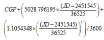 (1)
(1)
where JD = Julian day, 2000.0 = JD 2451545.0 = 12:00 UT January 01st 2000 and T = the number of Julian years (= 365.25 days) since 2000.0 i.e., (JD – 2451545.00)/365.25.
The second correction is to remove the prograde precession of the perihelion of the Earth’s orbit with respect to the stars. This is done using the following formula for the cumulative precession of the Perihelion (CPP) in degrees since the year 2000.0:
 (2)
(2)
Equation (2) is derived using a four-step process that is based upon the data that is generated by the Alcyone software program. First, the program is used to determine the longitude of the Earth’s perihelion every 12 hours in UT over the period from 2000 to 2550 AD. Second, the general precession (i.e., GP in arc seconds per Julian year) is calculated using equation (1) at the mid-point of each decade (e.g. the mid-point of the 2060’s is January 1st 00:00 UT 2065). Third, the longitudes of the perihelion that are generated by the program are used to calculate decadal mean precession of the perihelion with respect to the stars (DMPP), using the formula:
 (3)
(3)
where LPH=longitude of the perihelion in degrees for a heliocentric reference frame whose zero point is the Vernal Equinox. Finally, a second order polynomial fit is made to a plot of DMPP vs time (in years) which gives the rate of precession of the Perihelion with respect to the stars (in arc seconds per year) for all dates between 2000 and 2550 A.D. Thus, equation (2) is simply the cumulative sum of this precession rate, expressed in degrees per year.
Figure 2 shows a reproduction of Figure 1c. Points that are fixed with respect to a frame of reference that tracks with the precession of the Earth’s axis will lie along a horizontal line in this diagram. Superimposed upon this figure are diagonal coloured lines that show the drift of any point in this diagram that is fixed with respect to the Perihelion of the Earth’s orbit. The drift that is applied is simply the sum of the cumulative general precession (CGP = equation (1)) and the cumulative precession of Perihelion (CPP = equation (2)) measured in degrees since 2000.0. The drift per year varies from being 61.90 arc seconds in 2000 AD to 62.08 arc seconds in 2550 A.D.

Figure 2: Is a reproduction of Figure 1c. All points that are fixed with respect to a frame of reference that tracks with the precession of the Earth’s axis will lie along a horizontal line in this diagram. There are 12 diagonal coloured lines superimposed upon Figure 2 to show how 12 specific lunar alignment point would drift in a reference frame that is fixed with respect to the Perihelion of the Earth’s orbit (see the text for details about these alignment points and diagonal lines).
There are 12 diagonal coloured lines superimposed upon (Figure 2) to show how 12 given lunar alignment points would drift in a reference frame that is fixed with respect to the Perihelion of the Earth’s orbit.
An initial lunar alignment point (corresponding to time t = 0) is chosen on each diagonal line and then the drift line is used to determine the time elapsed since t = 0 for other lunar alignment points to reoccur at or near to the same relative point in the Earth’s orbit.
The 12 diagonal lines are grouped into three sequences. The initial point at t = 0 on the red line in the first sequence (solid lines) is set at the Vernal Equinox in 1993.25 A.D., while the initial points on each of subsequent lines in the sequence are spaced at intervals of 31 years at the Vernal Equinoxes in 2024.25, 2055.25, 2086.25, 2017.25 A.D. The initial point at t = 0 on the red line in the second sequence (short dashed lines) is set at the Vernal Equinox in 2002.25 A.D., while the initial points on each subsequent line are spaced at intervals of 31 years at the Vernal Equinoxes in 2033.25, 2064.25, 2095.25 A.D. Lastly, initial point at t = 0 on the red line in the third sequence (long dashed lines) is set at the Vernal Equinox in 2011.25 A.D., while the initial points on each subsequent line are spaced at intervals of 31 years at the Vernal Equinoxes in 2042.25 and 2073.25 A.D.
For each of the 12 sequences, an alignment index (ϕ) is defined to show how close a given lunar alignment point is to the point in the Earth’s orbit where the sequence’s initial lunar alignment point occurred:
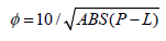 (4)
(4)
where P is the angle of a given lunar alignment point in degrees and L is the angle of the diagonal drift line, at the time of the lunar alignment. Note that ϕ is arbitrarily set to 10 at time = 0.
Figure 3 shows the mean value of ϕ versus the time in years since t = 0, for the 12 alignment sequences shown in Figure 2. Close inspection of the alignment peaks in Figure 3 show an alternating combination of 28.75 and 31.00-year cycles that leads to a repeating 208.0-year pattern.

Figure 3: The mean value of the lunar alignment index (ϕ) versus the time in years since t = 0, for the 12 alignment sequences shown in Figure 2. The most prominent alignment peaks in Figure 3 exhibit a 208-year repetition pattern, with each alignment peak appearing at a simple multiple of 59.79 (= 28.75 + 31.00) years plus 28.75 years. These peaks occur at simple half multiples of the Full Moon Cycle (FMC), as well i.e.: 0 × (28.75 + 31.00) + 28.75 years = 28.75 years ≈ 25.5 FMC’s; 1 × (28.75 + 31.00)+28.75 years = 88.5 years ≈ 78.5 FMC’s; 2 × (28.75 + 31.00) + 28.75 years = 148.25 years ≈ 131.5 FMC’s; 3 × (28.75 + 31.00) + 28.75 years = 208.0 years ≈ 184.5 FMC’s etc. it is important to note that the 208-year repetition pattern in the tidal alignments takes place no matter what starting Vernal Equinox is chosen. Hence, the 208-year repetition pattern appears to be ubiquitous in the tidal alignment record.
The detail of the 208-year repetition pattern is set out in Table 1. What this data shows are that the four strongest peaks in the repetition pattern are all simple multiple of 59.75 years (= 28.75 + 31.00) plus 28.75 years, as well as being simple half multiples of the Full Moon Cycle (FMC), such that:
0 × (28.75 + 31.00) + 28.75 years = 28.75 years ≈ 25.5 FMC’s
1 × (28.75 + 31.00) + 28.75 years = 88.5 years ≈ 78.5 FMC’s
2 × (28.75 + 31.00) + 28.75 years = 148.25 years ≈ 131.5 FMC’s
3 × (28.75 + 31.00) + 28.75 years = 208.0 years ≈ 184.5 FMC’s
[N.B. The Full Moon Cycle is the time required for the Perigee of the lunar orbit to realign with the Sun (= 411.7844303 days = 1.127428 tropical years).]
| Alignment | Increment in Years | Strength of Alignment |
|---|---|---|
| 0 | 0 | Perfect – by definition |
| 28.75 | 28.75 | Moderate – with a weaker peak at 31.00 years |
| 59.75 | 31.00 | Moderate – mixed with a peak at 62.00 years |
| 88.50 | 28.75 | Strong |
| 119.50 | 31.00 | Weak – mixed with equal peak at 117.25 years |
| 148.25 | 28.75 | Strong |
| 179.25 | 31.00 | Weak – mixed with equal peak at 177.0 years |
| 208.0 | 28.75 | Strong |
Table 1: The detail of the 208-year repetition pattern is set out.
In addition, it is evident that a simple extension of this 208-year repetition pattern produces alignment periods that match those of the other prominent peaks that appear in Figure 3: 236.75 (= 208.0 + 28.75) years; 296.50 (= 208.0 + 88.50) years; 356.25 (= 208.0 + 148.25) years; 416.0 (= 208.0 + 208.0) years; 444.75 (= 416.0 + 28.75) years; and 504.5 (= 416.0 + 88.5) years. Finally, it is important to note that the 208-year repetition pattern in the tidal alignments takes place no matter what starting Vernal Equinox is chosen. Hence, the 208-year repetition pattern appears to be ubiquitous in the tidal alignment record.
[N.B. This analysis tells us that if you started out with a New Moon at a time when the lunar-line-of-apse is pointing directly at the Sun near a seasonal boundary, after 207.99 sidereal years you will have a Full Moon at a time when the lunar line-of-apse points directly away from the Sun near the same seasonal boundary. Hence, this indicates that the full lunar alignment cycle (i.e., a return to a New Moon at a time when line-ofapse points directly at the Sun near the same seasonal boundary) is 416.0 years, rather than 208.0 years which is really just a half cycle.]
Results
The full significance of the 208-year repetition pattern in the periodicities of lunar alignments only becomes apparent when these periodicities are compared to those observed in the spectra for two proxy time series. The first period spectrum is displayed in Figure 4a. It shows the amplitude spectrum of the maximum daytime temperatures (Tm) on the Southern Colorado Plateau for a 2,264-year period from 266 BC to 1997 AD. This spectrum has been recreated from a digitization of part of Figure 3a [4]. Tm is believed to be a proxy for how warm it gets during the daytime in any given year i.e., it is an indicator of annual mean maximum daytime temperature. Tm is derived from the tree ring widths of Bristlecone Pines (P. aristata) located near the upper tree-line of the San Francisco Peaks (3,536 m). These trees were chosen because it is believed that their growth is primarily limited by the daily maximum temperature at this location. Spectral analysis of Tm identifies spectral peaks at 88 (Gleissberg cycle), 106, 130, 148, 209 (de Vries Cycle), 232, 353 and 500 years [5].

Figure 4: a) The amplitude spectrum of the maximum daytime temperatures (Tm) on the Southern Colorado Plateau for a 2,264-year period from 266 BC to 1997 AD. Prominent spectral peaks appear at 88 (Gleissberg cycle), 106, 130, 148, 209 (de Vries Cycle), 232, 353, 425 and 500 years; b) The Fourier spectrum of the solar modulation potential (ϕm) for the last 9400 years. ϕm is a proxy for the ability of the Sun’s magnetic field to deflect cosmic rays, and as such it is good indicator of the overall level of solar activity. It is derived from production rates of the cosmogenic radionuclides. Prominent spectral peaks appear at 88 (Gleissberg cycle), 104, 130, 150, 208 (de Vries cycle), 232, 351, 410?, 440 and 508 years; c) A reproduction of the lunar alignment index (i.e. ϕ) from Figure 3. Prominent alignment peaks occur at 88.5 (Gleissberg cycle), 148.25, 208.0 (de Vries cycle), 236.75, 296.5, 356.25, 416.0, 444.75, 504.5 years. Vertical dotted lines are used to compare the periods in this spectrum with those of the spectrum displayed above in Figures 4a and 4b.
The second period spectrum is displayed in Figure 4b. It shows the Fourier spectrum of the solar modulation potential (ϕm) for the last 9400 years. This spectrum has been recreated from a digitization of Figure 5a of [6]. ϕm is a proxy for the ability of the Sun’s magnetic field to deflect cosmic rays, and as such it is good indicator of the overall level of solar activity. It is derived from production rates of the cosmogenic radionuclides 10Be and 14C [7]. Spectral analysis of ϕm identifies spectral peaks at 88 (associated with the Gleissberg cycle - [8,9] 104, 130, 150, 208 (associated with the de Vries cycle – [7]), 232, 351, and 508 years [10,11],

Figure 5: The red curve is the de-trended amplitude of the semi-annual component of the polar fast Fourier transform (FFTP) of the LOD for each year from 1964 and 2014. The curve is constructed by taking the FFTP of the raw LOD data in a sliding four-year window and then extracting the magnitude of the semi-annual component from each spectrum. The blue curve is the de-trended annually averaged GCR hourly counting rates for Moscow between 1958 and 2010 [Note that the GCR hourly counting rates have been arbitrarily divided by 150,000 to roughly match the variance between these two curves]. Cross correlation analysis of the two curves shows that the GCR flux and the semiannual component of the Earth’s LOD are moderately correlated (correlation coefficient = 0.52). In addition, the comparison shows that the correlation is causal, with the changes in the GCR flux preceding those seen in the semiannual component of the Earth’s LOD by roughly one year.
Finally, Figure 4c shows the lunar alignment index (i.e. ϕ) from Figure 3. Vertical dotted lines are used to compare the periods in this spectrum with those of the spectrum displayed in Figures 4a and 4b. This comparison shows that, of the nine most prominent periods seen in Figure 4c (bold numerals in column 3 of Table 2), eight have closely matching peaks in the spectrum of solar modulation potential (ϕm – bold numerals in column 2 of Table 2). The one noticeable mismatch between these spectra occurs at 296.5 years. Similarly, of the nine most prominent periods seen in Figure 4c, seven have closely matching peaks in the spectrum of the maximum daytime temperatures (Tm highlighted in column 1 of Table 2). [N.B. It could be argued that the reduction in the number of close matches from eight to seven is just an artefact of the lower resolution of Tm spectrum, which merges the 416.0 and 444.75 year peaks to produce single peak at ~ 430 years.]. In addition, there are two peaks, one at 104 years (seen in both the ϕm and Tmspectra) and the other at 177 years (only seen in the Tm spectrum), which are either sub–multiples (i.e., 104.0 years = 208.0/2 years) or multiples (i.e., 177.0 years = 2.0 × 88.5 years) of other existing peaks.
| Maximum Daytime Temperature | Solar Modulation Potential | Lunar Alignment Index |
|---|---|---|
| 88 | 88 | 88.5 |
| 130 | 130 | ? |
| 148 | 150 | 148.25 |
| 209 | 208 | 208.0 |
| 232 | 232 | 236.75 |
| ? | ~ 285? | 296.5? |
| ~ 320 | ~ 327 | 327.5 |
| 353 | 351 | 356.25 |
| ~ 425 | ~ 410? | 416.0 |
| ~ 440 | 444.75 | |
| 500 | 508 | 504.5 |
Table 2: The fact that the periods of eight out of nine of the most prominent peaks in the lunar alignment spectrum (Highlighted column 3 of Table 2).
The fact that the periods of eight out of nine of the most prominent peaks in the lunar alignment spectrum (highlighted column 3 of Table 2) closely match those in the spectra of ϕm and Tm, strongly supports the contention that all three of these phenomena are closely related to one another. However, the exact form of this link is difficult to specify since there could be a direct causal link between two or more of these phenomena or there may be a common underlying factor that influences all three [10-13].
The solar connection between Tm and ϕm
A common underlying factor that could affect both Tm and ϕm is climate [14-16]. This comes about because the 10Be and 14C deposition rates could be significantly influenced by climatic variations. The problem with this hypothesis is that the deposition rates for 10Be and 14C have distinctly different dependences upon the various climate systems. This should be reflected in their long-term deposition rates. However, the variations of both radionuclides are strikingly similar on time scales longer than ~ 40 years, strongly implying that their longterm variations are not being primarily driven by climate effects [12,17-19]. Indeed, principal component analyses of the 10Be and 14C records show that, on multi-decadal to centennial time scales, the radionuclide production signal accounts for 76% of the total variance in the data [18,19]. This would imply that there is a causal link between Tm and near-Earth GCR flux, with a factor related to the latter driving the former.
One possible explanation for a causal link between ϕm and Tm is that the GCR flux hitting the Earth produce significant changes in the level of cloud cover that result in long term variations in the Earth’s mean temperature [20-22]. However, the chief problem with GCRcloud models of this type is that the existing multi-decadal satellitebased cloud datasets show no significant correlations between the total amounts of cloud cover on global scales and the levels of GCR fluxes hitting the Earth [23].
An implicit assumption that is used by those who reject GCR-cloud models is that the GCR flux hitting the Earth needs to produce changes in the total amount of cloud cover over the majority of the globe in order to significantly affect the world mean temperature. However, this assumption ignores the possibility that regional changes in the amount of cloud cover could influence the rate at which the Earth’s climate system warms or cools. Of course, for this to be true there would have to be observational evidence that shows that the GCR flux can affect the level of cloud cover on a regional scale.
Support for this hypothesis is provided [23] who claim that existing multi-decadal ground-based datasets for clouds show that there is a weak but significant correlation between the amounts of regional cloud cover and the overall level of GCR fluxes. In addition, Larken et al. [24] find that there is a strong and robust positive correlation between statistically significant variations in the short-term (daily) GCR ray flux and the most rapid decreases in cloud cover over the mid-latitudes (30° – 60° N/S). Moreover, [24] find that there is a direct causal link between the observed cloud changes and changes in the sea level atmospheric temperature, over similar time periods.
There also needs to be some evidence that changes in the amount and type of cloud cover on a regional scale can influence the efficiency with which the Earth warms and cools? Averaged over a full year, the difference between radiation received from the Sun and outgoing longwavelength radiation is positive equatorward and negative poleward of about 40° latitude [25]. This means that latitudinal gradient in annual mean net radiation absorbed by the climate system must be balanced by a poleward flux of energy and momentum. In addition, the vast bulk of the meridional energy and momentum transport above the Earth’s crust takes place in the atmosphere rather than the oceans, with most of the atmospheric transport resulting from the Hadley circulation in the tropics and sub-tropics, and jet-stream eddies in the higher midlatitudes [25]. The fundamental underlying cause for this meridional flux is the atmospheric temperature gradient between the tropics and the pole [26] find that the atmospheric temperature gradient between the tropics and the poles is enhanced by the meridional gradient of the atmospheric cloud effect. These authors show that this is primarily caused by the atmospheric cooling effects of low level cloud in the midlatitudes and the polar region. Overall [26] find that the meridional gradient of the cloud effect increases the rate of meridional energy transport.
Hence, it is entirely conceivable that long-term systematic changes in the amount and type of cloud cover at different latitudes, possibly caused by variations in the overall level of GCR, could lead to changes in the long-term poleward energy and momentum flux which, in turn, would lead to long-term changes in the rate at which the Earth warms and cools. If this is the case, then we would expect to see a correlation between the long-term changes in the GCR flux and a climate variable that is dependent upon the atmospheric temperature gradient between the tropics and the poles. One such climate variable is the average peak strength of the atmospheric zonal winds.
The vertical height of a given pressure surface within the atmosphere or geopotential height is given by:
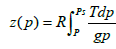 (5)
(5)
where z is the height in the atmosphere, p is the pressure, R is the Universal Gas Constant, T is the temperature, g = 9.8 m s-2, and ps is the surface pressure, such that z (ps) = 0. This means that the vertical height of a pressure surface is dependent upon the surface pressure and the average temperature below that surface, with most of the dependence being on the latter rather than the former. Consequently, the vertical height of a given pressure surface is lower near the poles, where air temperatures are colder, than it is near the equator, where the air temperatures are much warmer. These latitudinal gradients in the height of the pressure surfaces lead to a pressure gradient in the upper troposphere between the tropics and the poles. When this is combined with the Coriolis force associated with the rapid rotation of the Earth, it produces strong zonal winds. These winds blow in an easterly direction in the upper troposphere of the mid-latitudes of both hemispheres, with the strongest zonal wind speeds being found within the cores of the sub-tropical jets. Hence, the variations in the peak strength of the zonal atmospheric winds are fundamentally dependent upon both the variations in the Earth’s rotation rate and the variations in the temperature difference between the tropics and the poles.
Numerous studies show that annual and semi-annual changes in the speed of the zonal westerly winds are responsible for most of the variations that are seen in the annual and semi-annual component of the Earth’s length-of-day (LOD) [27-32]. The close correspondence between these two phenomena comes about because the total angular momentum of the Earth/Atmosphere system is effectively conserved over semi-annual to annual time scales [33].
Hence, if the long-term cooling and warming rates of the Earth are being influenced by GCR-induced regional cloud formation then there should be a correlation between variations seen in the semi-annual component of the Earth’s LOD and the GCR flux. Such a correlation is displayed in Figure 5.
The red curve in Figure 5 is the de-trended amplitude of the semiannual component of the polar fast Fourier transform (FFTP) of the LOD for each year from 1964 and 2014 as per International Earth Rotation and Reference Systems Service (IERS) [34]. The curve is constructed by taking the FFTP of the raw LOD data in a sliding fouryear window and then extracting the magnitude of the semi-annual component from each spectrum. The blue curve displayed in Figure 4 is the de-trended annually averaged GCR hourly counting rates for Moscow between 1958 and 2010 (NOAA - National Centers for Environmental Information [35]) [Note that the GCR hourly counting rates have been arbitrarily divided by 150,000 to approximately match the variance between these two curves].
Analysis of the two curves shows that the GCR flux and the semiannual component of the Earth’s LOD are moderately correlated (correlation coefficient=0.52. Moreover, the comparison shows that the correlation is causal, with the changes in the GCR flux preceding those seen in the semi-annual component of the Earth’s LOD by roughly one year. This result is in general agreement with [32] who find that there is an excellent correlation between the de-trended GCR flux and the semi-annual component of the Earth’s LOD, although they do not find any systematic causal lag between the two parameters.
It is important to note that while there appears to be a correlation between the de-trended GCR flux and the semi-annual component of the Earth’s LOD, this does not mean that the GCR-induced regional cloud formation is the cause. All this correlation tells us is that there is some, as yet, unknown factor associated with the Sun that is influencing the semi-annual component of the Earth’s LOD and that factor is correlated with the de-trended GCR.
Hence, the solar connection between Tm and ϕm can be summarized using a heuristic luni-solar model like that shown in Figure 6. Firstly, the model proposes that there must be some, as yet, unknown factor associated with the level of solar activity on the Sun (e.g. possibly the overall level GCR hitting the Earth) that is producing long-term systematic changes in the amount and/or type of regional cloud cover. Secondly, the model proposes that the resulting changes in regional cloud cover lead to variations in the temperature differences between the tropics and the poles which, in turn, result in changes to the peak strength of the zonal tropical winds. Thirdly, the model further proposes that it is the long-term changes in the amount and/or type of regional cloud cover, combined with the variations in the temperature differences between the tropics and the poles that lead to the long-term changes in the poleward energy and momentum flux. And finally, the model proposes that it is this flux which governs the rate at which the Earth warms and cools, and hence, determines the long-term changes in the world mean temperature.

Figure 6: The Luni-Solar Model puts forward a number of proposals in order to explain the connections between ϕ, Tm and ϕm. Refer to the text for the details about these proposals.
A model of this nature has the added advantage that it produces an apparent correlation between the semi-annual component of the Earth’s LOD and the GCR flux because of the strong coupling between the peak strength of the zonal tropical winds and LOD. As stated previously, this coupling is a direct result of the conservation of the total angular momentum of the Earth/Atmosphere system, over semiannual to annual time scales.
The connection between the lunar tidal cycles and Tm
Figure 7 shows the real part of the polar fast Fourier transform of the Earth’s daily LOD values over a 54-year period between January 1st 1962 and June 5th 2016. The data used in this plot is available online from the International Earth Rotation and Reference Systems Service (IERS) [34].

Figure 7: The real part of the polar fast Fourier transform of the Earth’s daily LOD values over a 54-year period between January 1st 1962 and June 5th 2016. The LOD spectrum is dominated five spectral peaks that include: the annual variation (= 365.24 days); the semi-annual variation (= 182.62 days); the anomalist month (= 27.55 days); the semi-Tropical and semi-Sidereal month (= 13.66 days); and the semi-Draconic month (= 13.61 days).
The LOD spectrum in Figure 7 is dominated five spectral peaks that include: the annual variation (= 365.24 days); the semi-annual variation (= 182.62 days); the anomalist month (= 27.55 days); the semi-Tropical and semi-Sidereal month (= 13.66 days); and the semi-Draconic month (= 13.61 days).
The peaks associated with the annual and semi-annual variations in the Earth’s LOD result from changes in the angular momentum of the Earth that are a response to the slow seasonal variations in the latitudinal location and strength of the Earth's zonal winds. In contrast, the three prominent lunar peaks are produced by the movement the atmospheric and oceanic tidal bulges across the Earth’s equatorial and tropical regions over each lunar monthly cycle.
The first peak, which is associated with the anomalistic lunar month, results from the Moon moving from Perigee to Perigee of its lunar orbit, producing a 27.55-day modulation in the strength of the tidal bulges and their effect upon the Earth’s LOD. The second peak, which is associated with the semi-Tropical lunar month, results from the tidal bulges in the Earth’s atmosphere and oceans moving from their most northerly/southerly latitude, across the Earth’s equator, to their most southerly/northerly latitude, once every 13.66 days (≈ one semi-Sidereal month). This semi-monthly motion of the tidal bulges increases and then decreases the Earth’s LOD by about~1 millisecond [36]. Of course, it is immediately followed by an increase and then decrease in LOD of roughly the same order of magnitude, as the Moon moves from its most southerly/northerly to its most northerly/ southerly latitude, over the next consecutive semi-Tropical month. Finally, the third peak, which is associated with the Draconic lunar month, results from the Moon moving from one its orbital nodes to the other, once every 13.61 days. This particular peak is associated with monthly movement of the tidal bulges in the Earth’s atmosphere and oceans above and below the point where the Ecliptic crosses the Earth’s equator. This is caused by the 5.15O tilt of the lunar orbit with respect to the Ecliptic.
The close matches between the periods of the prominent peaks that are seen in spectra of ϕ Figure 4a and Tm Figure 4c, indicate that a factor associated with the times at which the Perigee of the lunar orbit points directly towards or directly away from the Sun, at times when the Earth is at one of its Solstices or Equinoxes, has an influence on the Earth’s mean temperature [N.B. these alignments take place in frame of reference that is fixed with respect to the Perihelion of the Earth’s orbit].
The Luni-Solar Model shown in Figure 6 suggests one possible mechanism that might explain this influence. This model proposes that the alignment between the times when the Perigee of the lunar orbit points directly towards or directly away from the Sun (i.e., at ½ multiples of the FMC) and the annual and semi-annual variation in the Earth’s LOD (which are synchronised with the seasonal boundaries), could produce long term periodicities in the zonal wind speeds of the Earth’s atmosphere that match those seen in ϕ. These wind speed changes, in turn, would produce long-term periodicities in the Earth’s mean temperature through their influence upon the efficiency with which the Earth warms and cools.
It is important to note that the proposed mechanism is not just simply one where the semi-annual variation in LOD is being modulated by some multiple of the anomalistic month. Indeed, the close matches between the periods of the prominent peaks that are seen in Figures 4a and 4c allows us to place very specific constraints upon the underlying lunar tidal mechanism involved. These specific constraints will be used to further investigate the proposed luni-solar tidal mechanism in paper two of this series. They include that the mechanism:
a) It must be associated with the periodic alignments of the lunar line-of-apse with the Earth-Sun line once every 205.89 days (= ½ of a FMC) and how well these events align with the seasons (i.e., the Solstices and Equinoxes).
b) It must operate in frame-of-reference that is fixed with respect to the Perihelion of the Earth’s orbit.
c) It is not associated with the lunar phase cycle, since alignments of New/Full Moons with the Perigee of the lunar orbit, that align with the seasons, have long-term periodicities of 31.0, 62.0, 93.0, and 186.0 years, which are not the periodicities that are seen in Figures 4a and 4c.
d) It is not connected with the alignment of the 18.6/9.3- year Draconic cycle with the seasons, since these alignments have a periodicity of 46.5, 93.0, 139.5, 186.0, and 232.5 years. Again, these are not the periodicities that are seen in Figures 4a and 4c.
e) It is not linked to the periodic alignments of the lunar lineof- apse with the lunar line-of-nodes and how these alignments resynchronize with the seasons. An alignment of the line-of-apse and the line-of-nodes takes place roughly once every 5.997 tropical year, and so it will slowly drift out of synchronization with the seasons, taking ≈ 496 tropical years to move from being synchronized with one equinox/ solstice to being synchronized with the next solstice/equinox.
The connection between the lunar tidal cycles (ϕ) and ϕm
Perhaps the most bizarre result that has come out of this study is the fact that, of the nine most prominent periods seen in the lunaralignment time series (ϕ - Figure 4c), eight have closely matching peaks in the spectrum of solar modulation potential (ϕm – Figure 4b). One explanation for this synchronicity is that there is an underlying mechanism that is responsible for both the long-term periodicities that are seen in the alignment of the Lunar Perigee-Syzygies with the seasons, as well as the long-term periodicities that are observed in the overall level of the Sun’s magnetic activity.
There are many papers claiming that there is a link between the orbital motions of the planets and the overall level of solar activity in the outer layers of the Sun. Indeed, there have been so many papers written on this topic that it is very difficult to list them all here. However, a good review of the extensive literature on this topic is given by Scafetta [37] and Wilson [38] in the Special Edition of the Pattern Recognition in Physics [39].
One model that has been put forward to explain the observed link between the orbital periods of the planets and the level of the Sun’s magnetic activity is the Venus–Earth–Jupiter (VEJ) tidal-torqueing model [38]. This model is based on the idea that Jupiter applies the dominant gravitational force acting upon the outer convective layers of the Sun and that, excluding Jupiter, the planets that apply the dominant tidal forces upon the convective layers are Venus and the Earth.
The VEJ tidal-torqueing model proposes that periodic alignments of Venus and the Earth on the same or opposite sides of the Sun produce temporary tidal bulges. It further proposes that Jupiter’s gravitational force tugs upon these tidally-induced asymmetries and either slows down or speeds-up the rotation rate of the plasma at the base of the outer convective layers of the Sun. The model claims that it is these variations in the rotation rate of the plasma at the base of the convective layer of the Sun that modulate the Babcock–Leighton solar dynamo, leading to the observed long-term changes in the overall level of solar activity.
Further empirical evidence to support the VEJ tidal-torqueing model is provided by equation 6 [37,40].
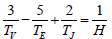 (6)
(6)
where TV = the sidereal orbital period of Venus = 0.615187 sidereal years
TE = the sidereal orbital period of the Earth = 1.000000 sidereal years
TJ = the sidereal orbital period of Jupiter = 11.862408 sidereal years and H = the Hale sunspot cycle period = 22.141 sidereal years.
[N.B. The planetary periods that are used in these calculations are TJ = 4332.82 days, TS = 10755.698 days, TV = 224.70080 days and TE = 365.256363 days, with the length of the tropical year being equal to 365.2421897 days. The periods for Venus, Jupiter and Saturn are those used to generate ephemeris at the JPL Horizon web interface [41] located.
Equation 6 provides a simple expression linking the sidereal orbital periods of the planets Venus, Earth and Jupiter to a period of time that closely matches the length of the Hale sunspot cycle (Wilson 2011). Indeed, the value of 22.14 years just happens to be the time required for Jupiter to move through 180 degrees of arc about the Sun, with respect to a line that is formed by the periodic alignments of Venus and the Earth, once every 0.79933 sidereal years.
If we accept the possibility that planetary gravitational and tidal forces could influence the overall level of the Sun’s magnetic activity then the synchronicity between ϕ with ϕm in Figures 4b and 4c could be explained if these same planetary forces played a role in shaping the present-day orbit of the Moon.
It is known that the weak tidal forces of the planets Venus, Mars and Jupiter have continuously moulded and shaped the Moon’s orbit. If we couple this with the fact that the Moon has slowly receded from the Earth over the last 4.6 billion years, there must have been times when the orbital periods of Venus, Mars and Jupiter have been in resonance with the precession rate of the line-of-nodes and the lineof- apse of the lunar orbit [42]. When these resonances have occurred, they would have greatly amplified the effects of the planetary tidal forces upon the lunar orbit [42]. Hence, any observed synchronization between the precession rates for the line-of-nodes and the line-of-apse of the lunar orbit and the orbital periods of these planets, would simply be a cumulative fossil record of these historical resonances [43].
Hence, if there is some common underlying mechanism that is responsible for synchronizing ϕ with ϕm then there should also be a simple mathematical expression that links the orbital periods of the planets with the orbit of the Moon. Such an expression is provided by equation 7:
 (7)
(7)
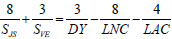
This equation shows that there is direct link between the synodic period of Jupiter and Saturn (= 19.864691 sidereal years) and the synodic period of Venus and Earth (= 1.598662 sidereal years) with three canonical periods that are associated with the lunar orbit. The first is the Draconic Year (DY = 0.948977 sidereal years), which is the time required for one of the nodes of the lunar orbit to realign with the Sun. The second is the Lunar Nodical Cycle (LNC = 18.599203 sidereal years), which is the time required for the lunar line-of-nodes to precess once around the Earth with respect to the stars. The third is the Lunar Anomalistic Cycle (LAC = 8.850237 sidereal years), which the time required for the lunar line-of-apse to precess once around the Earth with respect to the stars.
Taking the harmonic mean of ½ × LNC and the LAC (= 9.069 sidereal years), it is possible to rearrange equation 7 to get:
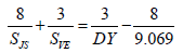 (8)
(8)
Equation 8 directly connects the synodic periods of Jupiter/ Saturn and Venus/Earth with the Draconic Year and a period of time ≈ 9.1 sidereal years. Interestingly, this closely matches the period of a prominent peak that is seen in the spectra of the world’s mean HadCRUT3/4 temperatures that [44-47] attribute to lunar tidal effects upon temperature.
Hence, it is not beyond the realm of possibilities that the synchronicities seen between the ϕ and ϕm are simply a result of the fact that both are influenced by the orbital configuration of the planets [48].
Discussion and Analysis
Lunar ephemeris data is used to find all the times when the Perigee of the lunar orbit points directly at, or away, from the Sun, at times when the Earth is located at one of the cardinal points of its seasonal calendar (i.e., the summer solstice, winter solstices, spring equinox or autumnal equinox). All of the close lunar alignments are identified over a 536-year period between January 1st 1993 A.D. 00:00 hrs UT and December 31st 2528 A.D 00:00 hrs UT.
When a plot is made of the precision of these alignments, in a frame-of-reference that is fixed with respect to the Perihelion of the Earth’s orbit, the most precise alignments take place in an orderly pattern that repeats itself once every 208.0 years:
0 × (28.75 + 31.00) + 28.75 years = 28.75 years ≈ 25.5 FMC’s
1 × (28.75 + 31.00) + 28.75 years = 88.5 years ≈ 78.5 FMC’s
2 × (28.75 + 31.00) + 28.75 years = 148.25 years ≈ 131.5 FMC’s
3 × (28.75 + 31.00) + 28.75 years = 208.0 years ≈ 184.5 FMC’s
A simple extension of this pattern gives additional precise alignments at periods of: 236.75, 296.50, 356.25, 416.0, 444.75 and 504.5 years. The full significance of the 208-year repetition pattern in the periodicities of lunar alignment index (ϕ) only becomes apparent when these periodicities are compared to those observed in the spectra for two proxy time series.
The first is the amplitude spectrum of the maximum daytime temperatures (Tm) on the Southern Colorado Plateau for a 2,264-year period from 266 BC to 1997 AD. Tm is believed to be a proxy for how warm it gets during the daytime in any given year i.e., it is an indicator of annual mean maximum daytime temperature. Tm is derived from the tree ring widths of Bristlecone Pines (P. aristata) located near the upper tree-line of the San Francisco Peaks (<3,536 m).
The second is the Fourier spectrum of the solar modulation potential (ϕm) for the last 9400 years. ϕm is a proxy for the ability of the Sun’s magnetic field to deflect cosmic rays, and as such it is good indicator of the overall level of solar activity. It is derived from production rates of the cosmogenic radionuclides 10Be and 14C. When a comparison is made between these three spectra it shows that, of the nine most prominent periods seen in the lunar alignment index, eight have closely matching peaks in the spectrum of solar modulation potential (ϕm), and seven have closely matching peaks in the spectrum of the maximum daytime temperatures (Tm). The fact that the so many of the most prominent peaks that are seen in the lunar alignment index spectrum closely match those seen in the spectra of ϕm and Tm, strongly supports the contention that all three of these phenomena are closely related to one another.
The critical piece of observational evidence that explains why Tm might be related to ϕm is provided [32]. These authors find that there is a good correlation between the de-trended GCR flux and the semiannual component of the Earth’s LOD. Our analysis confirms the correlation found [32] and shows that the correlation is causal, with the changes in the GCR flux preceding those seen in the semi-annual component of the Earth’s LOD by roughly one year.
This result leads us to develop a heuristic luni-solar model in order to explain the connection between Tm and ϕm. Firstly, the model proposes that there must be some, as yet, unknown factor associated with the level of solar activity on the Sun (e.g. possibly the overall level GCR hitting the Earth) that is producing long-term systematic changes in the amount and/or type of regional cloud cover. Secondly, it proposes that the resulting changes in regional cloud cover lead to variations in the temperature differences between the tropics and the poles which, in turn, result in changes to the peak strength of the zonal tropical winds. Thirdly, the model proposes that it is the long-term changes in the amount and/or type of regional cloud cover, combined with the variations in the temperature differences between the tropics and the poles that lead to the long-term changes in the poleward energy and momentum flux. And finally, it proposes that it is this flux which governs the rate at which the Earth warms and cools, and hence, determines the long-term changes in the world mean temperature.
The close matches between the periods of the prominent peaks that are seen in spectra of ϕ Figure 4a and Tm Figure 4c, indicate that a factor associated with the times at which the Perigee of the lunar orbit points directly towards or directly away from the Sun, at times when the Earth is at one of its Solstices or Equinoxes, has an influence on the Earth’s mean temperature [N.B. these alignments take place in frame of reference that is fixed with respect to the Perihelion of the Earth’s orbit].
Conclusion
The proposed Luni-Solar Model suggests one possible mechanism that might explain the influence of ϕ upon Tm. This model proposes that the periodicities associated with the long-term alignments between the times when the Perigee of the lunar orbit points directly towards or directly away from the Sun (i.e., half multiples of the FMC) and the seasons (i.e., the Solstices and Equinoxes – which, by definition, are synchronized with annual and semi-annual variations in LOD), produce comparable periodicities in the zonal wind speeds of the Earth’s atmosphere. These wind speed changes in turn produce longterm periodicities in the Earth’s mean temperature through their influence upon the efficiency with which the Earth warms and cool
Finally, if we accept the hypothesis that planetary gravitational and tidal forces could influence the overall level of the Sun’s magnetic activity, then the observed synchronicity between ϕ and ϕm could be explained if these same planetary forces played a role in shaping the present-day orbit of the Moon.
Acknowledgment
One of the authors (IW) would like to thank Mr. Ian A. Wilson and Mrs Marion N. Wilson for making the preparation of this paper possible.
Conflict of Interest
No outside funding was used to conduct this work. No conflicts of interest are involved.
References
- Capitaine N, Wallace P T, Chapront P (2003) Expressions for IAU 2000 precession quantities. Astron. & Astrophys. 412: 567-586.
- Chapront-Touz M, Chapront J (1991) Lunar tables and programs from 4000 B. C. to A.- D. 8000. Willmann-Bell, Richmond VA, USA.
- Ron C, Chapanov Y, Vondrak J (2012) Solar excitation of bicentennial earth rotation oscillations. Geomater 9: 259-268.
- Salzer MW, Kipfmueller KF (2005) Reconstructed temperature and precipitation on a millennial timescale from tree-rings in the Southern Colorado Plateau, USA. Climatic Change 70: 465–487.
- Abreu J A, Beer J, Ferriz-Mas A, McCracken KG, Steinhilber F (2012) Is there a planetary influence on solar activity? Astron. & Astrophys 548: A88.
- Stuiver M, Braziunas TF (1993) Sun, ocean, climate and atmospheric 14CO2: An evaluation of causal and spectral relationships. Holocene 3: 289-305.
- Gleissberg W (1944) A table of secular variations of the solar cycle. Terrestrial Magnetism and Atmospheric Electricity 49: 243-244.
- Damon PE, Sonnet CP (1991) The sun in time. University of Arizona Press, Tucson, AZ, pp: 360-388.
- McCracken KG, Beer JF, Steinhilber J, Abreu A (2013) Phenomenological study of the cosmic ray variations over the past 9400 years, and their implications regarding solar activity and the solar Dynamo. Solar Physics 286: 609-327.
- Steinhilber F, Beer J (2013) Prediction of solar activity for the next 500 years. Journal of Geophysical Research. Space Physics pp: 118: 1-7.
- Beer J, McCracken K, Von Steiger R (2012) Cosmogenic radionuclides: Theory and applications in the terrestrial and space environments: Springer, Berlin.
- Pedro JB, McConnell JR, Van Ommen TD, Fink D, Curran MAJ, et al. (2012) Solar and climate influences on ice core 10Be records from Antarctica and Greenland during the neutron monitor era. Earth and Planetary Science Letters. 355-356: 174–186.
- Nikitina I, Stozhkova Y, Okhlopkovb V, Svirzhevskya N (2005) Do Be-10 and C-14 give us the information about cosmic rays in the past:29th International Cosmic Ray Conference, Pune, 101-104.
- Hanslmeier A, Brajša R (2010) The chaotic solar cycle I. Analysis of cosmogenic 14C-data. Astron & Astrophys pp: 509: A5
- Hanslmeier A, Brajša R, Calogovic´ J, Vršnak B, Ruždjak D, et al. (2013) The chaotic solar cycle II. Analysis of cosmogenic 10Be data, Astron. & Astrophys. 550: A6
- Beer J, McCracken KG, Abreu J, Heikkilá U, Steinhilber F (2007) Proceedings of the 30th International Cosmic Ray Conference: Merida, Mexico.
- Abreu JA (2009) 10 Be in polar ice cores and 14C in tree rings: Separation of production and climate effects: PhD Thesis p: 46.
- Abreu JA, Beer J, Steinhilber F, Christl M, Kubik PW (2013) Be in ice cores and 14C in tree rings: separation of production and climate effects. Space Sci Rev1: 343-349.
- Svensmark H (1998) Influence of cosmic rays on the earth’s climate. Phys Rev Lett 81: 5027
- Svensmark H (2007) Cosmoclimatology: A new theory emerges. Astronomy & Geophysics 48: 18-24.
- Svensmark H, Bondo T, Svensmark J (2009) Cosmic ray decreases affect atmospheric aerosols and clouds. Geophys Res Lett 36: L15101.
- Laken BA, Pallé E, Čalogović J, Dunne EM (2012) A cosmic ray-climate link and cloud observations. J Space Weather Space Clim 2: A18.
- Laken BA, Kniveton DR, Frogley MR (2010) Cosmic rays linked to rapid mid-latitude cloud changes, Atmos Chem Phys 10: 10941-10948.
- Marshall J, Plumb RA (2008) Atmosphere, ocean and climate dynamics: an introductory text: Volume 93 of the International Geophysics Series: Elsevier, Academic Press. ISBN 978-0-12-558691-7
- Kato S, Rose FG, Rutan D A, Charlock TP (2008) Cloud effects on the meridional atmospheric energy budget estimated from cluds and the earth’s radiant energy system (CERES) Data. Journal of Climate 21: 4223 -4241.
- Rosen RD (1993) The axial momentum balance of Earth and its fluid envelope. Surv Geophysics 14: 1-29.
- Höpfner J (1998) Seasonal variations in length of day and atmospheric angular momentum. Geophys J Int135: 407-437.
- Höpfner J (2000) Seasonal length-of-day changes and atmospheric angular momentum oscillations in their temporal variability. J Geodesy 74: 335-358.
- Gross RS (2007) Earth rotation variations – Long period, in physical geodesy. T.A. Herring, (eds) Treatise on Geophysics, Vol. 11: Elsevier,  Amsterdam, The Netherlands.
- Sidorenkov NS (2009) The interaction between Earth’s rotation and geophysical processes. Weinheim: Wiley-VCH Verlag GmbH & Co. KGaA, Weinheim, Germany, p: 317.
- Le Mouël JL, Blanter E, Shnirman M, Courtillot V (2010) Solar forcing of the semiâ€annual variation of lengthâ€ofâ€day. Geophy Res Lett 37: L15307
- Hide R, Birch NT, Morrison LV, Shea DJ, White AA (1980) Atmospheric angular momentum fluctuations and changes in the length of the day. Nature 286: 114–117
- International Earth Rotation and Reference Systems Service (IERS) Earth Orientation Parameters (EOP) 08 C04 (IAU1980).
- Sidorenkov NS (2016) Celestial mechanical causes of weather and climate change. Atmospheric and Oceanic Physics. 52: 667-682.
- Scafetta N (2014) The complex planetary synchronization structure of the solar system. Pattern Recogn. Phys. 2: 1-19.
- Wilson IRG (2013) The Venus–Earth–Jupiter spin–orbit coupling model. Pattern Recogn Phys 1: 147-158.
- Mörner NA, Tattersall R, Solheim JE (2013) Pattern in solar variability, their planetary origin and terrestrial impacts. Pattern Recogn Phys 1: 203-204.
- Cuk M (2007) Excitation of lunar eccentricity by planetary resonances. Science. 318 :244
- Wilson IRG (2011) Are changes in the earth’s rotation rate externally driven and do they affect climate? The General Science Journal p:  3811.
- Scafetta N (2010) Empirical evidence for a celestial origin of the climate oscillations and its implications. J Atmos Sol Terr Phy 72: 951–970.
- Scafetta N, Willson RC (2013) Multiscale comparative spectral analysis of satellite total solar irradiance measurements from 2003 to 2013 reveals a planetary modulation of solar activity and its non-linear dependence on the 11yr solar cycle. Pattern Recogn Phys 1: 123-133.
- Solheim JE. (2013) Signals from the planets, via the Sun to the Earth. Pattern Recogn Phys 1: 177-184.
- Scafetta N (2014) Discussion on the spectral coherence between planetary, solar and climate oscillations: a reply to some critiques. Astrophys Space Sci 354: 2111.
- Wilson IRG (2014) Are the strongest lunar perigean spring tides commensurate with the transit cycle of Venus? Pattern Recogn Phys 2: 75-93.
- Sidorenkov NS (2015) Synchronization of terrestrial processes with frequencies of the Earth-Moon-Sun system. Odessa Astronomical Publications 28: 295-298.
Citation: Wilson IRG, Sidorenkov NS (2018) A Luni-Solar Connection to Weather and Climate I: Centennial Times Scales. J Earth Sci Clim Change 9: 446. DOI: 10.4172/2157-7617.1000446
Copyright: © 2018 Wilson IRG, et al. This is an open-access article distributed under the terms of the Creative Commons Attribution License, which permits unrestricted use, distribution, and reproduction in any medium, provided the original author and source are credited.
Select your language of interest to view the total content in your interested language
Share This Article
Recommended Journals
Open Access Journals
Article Tools
Article Usage
- Total views: 5088
- [From(publication date): 0-2018 - Dec 08, 2025]
- Breakdown by view type
- HTML page views: 4129
- PDF downloads: 959