Research Article Open Access
Analysis of Temperature Distribution through Rectangular Convective Fin Using Analytical Methods
1Mechanical Engineering Department, Amirkabir University of Technology, Tehran, Iran
2Mechanical Engineering Department, Babol Noshirvani University of Technology, Babol, Iran
- Corresponding Author:
- Ganji DD
Mechanical Engineering Department
Babol Noshirvani University of Technology, P.O. Box 484, Babol, Iran
Tel: +98 111 32 34 501
E-mail: ddg_davood@yahoo.com
Received Date: September 26, 2016; Accepted Date: November 01, 2016; Published Date: November 07, 2016
Citation: Mokhtarpour K, Ganji DD (2016) Analysis of Temperature Distribution through Rectangular Convective Fin Using Analytical Methods. Innov Ener Res 5:146.
Copyright: © 2016 Mokhtarpour K, et al. This is an open-access article distributed under the terms of the Creative Commons Attribution License, which permits unrestricted use, distribution, and reproduction in any medium, provided the original author and source are credited.
Visit for more related articles at Innovative Energy & Research
Abstract
In this paper, the power of the recently introduced method of Akbari-Ganji has been validated by solving two different nonlinear equations. In the first section, the temperature distribution model of a convective straight fin is found by solving the governing energy balance equation with Akbari-Ganji’s Method. The authenticity of this method has been checked considering the fourth-order Runge-Kutta. In the second section, a linear differential equation without enough boundary conditions is converted into a nonlinear differential equation with enough boundary conditions by derivation. The precision of the AGM method has been compared with two other semianalytical methods. Results were prepared for the ultimate solution function and its first derivative in both sections. The variational iteration method and the homotopy perturbation method were the ones which showed the lowest and the highest error amounts, respectively. The AGM method is also considered as an acceptable method with negligible error in solving different nonlinear equations.
Keywords
Rectangular convective fin; Akbari-Ganji’s Method (AGM); HPM; VIM; Fourth-order Runge-Kutta numerical method
Temperature Distribution Solution inside the Convective Straight Fin
Introduction
In the study of heat transfer, fins are surfaces extending from an object to increase the rate of heat transfer to or from the environment by increasing convection. Increasing the temperature gradient between the object and the environment, increasing the coefficient of convection heat transfer, or increasing the surface area of the object increases the heat transfer. Sometimes it is not feasible or economical to change the first two options. Thus, adding a fin to an object increases the surface area and can sometimes be an economical solution to heat transfer problems. The sketch of the convective straight fin is depicted (Figure 1).

Figure 1: The sketch of the rectangular convective straight fin under discussion.
Analyzing the fin problem consists of two sections. One is based on thermal convection through fin surface area and the other is based in thermal conduction through fin cross section. The one-dimensional energy balance equation governing the fin problem is as below:
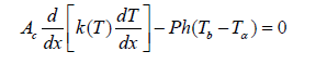 (1)
(1)
A linear temperature function for the thermal conductivity of the fin material is considered as below:
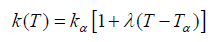 (2)
(2)
Where ka and k are the thermal conductivity at the ambient fluid temperature of the fin and the thermal conductivity variation, respectively. Employing the following dimensionless parameters [1-2]:
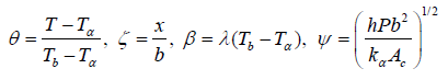 (3)
(3)
Therefore, the governing equation will reduce to:
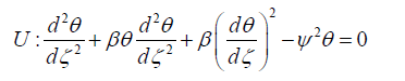 (4)
(4)
The corresponding boundary conditions are as below:
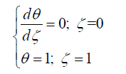 (5)
(5)
The heat transfer dissipation rate from the fin is expressed as below according to the Newton’s law of cooling:
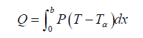 (6)
(6)
The fin efficiency which is defined as the ratio of actual heat transfer from the fin surface to the other side while the whole fin surface stays at the same temperature:
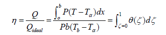 (7)
(7)
AGM approach
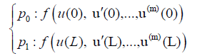
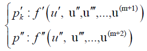
Description of the method: To elucidate on, consider the nonlinear differential equation p that is a function of the parameter u (a function of x) and its derivatives as below:
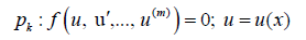 (8)
(8)
The corresponding boundary conditions are as below:
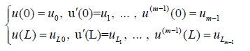 (9)
(9)
In order to solve the first differential equation with respect to the boundary conditions in x=L (Eq. 9), the corresponding answer is considered as follows:
 (10)
(10)
By means of increasing the number of series in Eq. 10, the obtained solution is closer to the real answer and shows more precision. Approximately, five or six sentences are enough for obtaining answers with negligible errors in applied problems. The boundary conditions are applied to the functions as below:
a) The application of the boundary conditions for the answer of differential Eq. 11 is in the form of:
If x=0
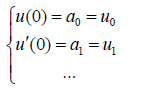 (11)
(11)
And if x=L
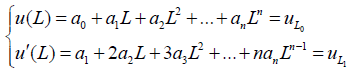 (12)
(12)
b) After substituting Eq. 12 into Eq. 8, the boundary conditions are applied on Eq. 8 according to the procedure below:
 (13)
(13)
With regard to the choice of n; n<m sentences from Eq. 10 and in order to make a set of equations which is consisted of (n+1) equations and (n+1) unknowns, we confront with a number of additional unknowns which are indeed the same coefficients of Eq. 10. Therefore, to remove this problem, we should derive m times from Eq. 8 according to the additional unknowns in the afore-mentioned sets of differential equations and then applying the boundary conditions on them.
 (14)
(14)
a) Application of the boundary conditions on the derivatives of the differential equation Pk in Eq. 14 is done in the form below:
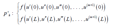 (15)
(15)
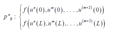 (16)
(16)
(n+1) equations can be made from Eq. 11-16 so those (n+1) unknown coefficients of Eq. 10 a0, a1, a2, … an can be computed. The answer of the nonlinear differential Eq. 8 will be obtained by computing coefficients of Eq. 10.
Applying AGM to the given equation: The answer of the energy balance equation governing the fin problem can be considered as a finite series of polynomials with constant coefficients:
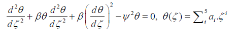 (17)
(17)
The aforementioned unknown coefficients are capable of being computed by applying the boundary conditions.
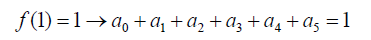
a) Applying the boundary conditions on Eq. 17:
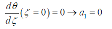 (18)
(18)
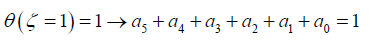 (19)
(19)
b) Applying the boundary conditions on the main differential Eq. 4 and its derivatives:
 (20)
(20)
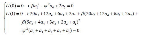 (21)
(21)
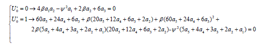 (22)
(22)
By solving a set of algebraic equations, six unknown coefficients are computed according to the existing six equations. By entering the values of the coefficients, the ultimate answer of AGM method is obtained [12-20].
Results and Conclusion
The Temperature Distribution tables and figures are depicted below for two cases in which the dimensionless parameter β describing variation of thermal conductivity is considered zero which corresponds to a constant thermal conductivity through the fin’s material (Tables 1 and 2; Figures 2 and 3).
| ζ | β=0, Ψ=0.5 | ||
|---|---|---|---|
| AGM | Numerical | Error | |
| 0 | 0.648414986 | 0.648054499 | 0.000360487 |
| 0.1 | 0.651659539 | 0.651297468 | 0.000362071 |
| 0.2 | 0.661423401 | 0.661058833 | 0.000364568 |
| 0.3 | 0.677799078 | 0.677436294 | 0.000362783 |
| 0.4 | 0.700944784 | 0.700593758 | 0.000351026 |
| 0.5 | 0.731087896 | 0.730762995 | 0.000324901 |
| 0.6 | 0.768528415 | 0.768245949 | 0.000282466 |
| 0.7 | 0.813642421 | 0.813417762 | 0.000224659 |
| 0.8 | 0.866885533 | 0.866730522 | 0.000155011 |
| 0.9 | 0.928796369 | 0.928717806 | 7.86E-05 |
| 1 | 1 | 1 | 0 |
Table 1: The results of AGM and the fourth-order Runge-Kutta for Θ(ζ).
| ζ | β=0, Ψ=1 | ||
|---|---|---|---|
| AGM | Numerical | Error | |
| 0 | 0.886827894 | 0.886818904 | 8.99E-06 |
| 0.1 | 0.887936656 | 0.887927655 | 9.00E-06 |
| 0.2 | 0.891265668 | 0.891256693 | 8.98E-06 |
| 0.3 | 0.896823156 | 0.896814335 | 8.82E-06 |
| 0.4 | 0.904622907 | 0.904614478 | 8.43E-06 |
| 0.5 | 0.914684345 | 0.914676629 | 7.72E-06 |
| 0.6 | 0.927032599 | 0.927025948 | 6.65E-06 |
| 0.7 | 0.941698575 | 0.941693312 | 5.26E-06 |
| 0.8 | 0.958719023 | 0.958715403 | 3.62E-06 |
| 0.9 | 0.978136613 | 0.978134783 | 1.83E-06 |
| 1 | 1 | 1 | 9.99E-16 |
Table 2: The results of AGM and the fourth-order Runge-Kutta for Θ(ζ).

Figure 2: Comparison of the solutions via AGM and the fourth-order Runge- Kutta for Θ(ζ)–β=0, Ψ=0.5

Figure 3: Comparison of the solutions via AGM and the fourth-order Runge- Kutta for Θ(ζ)–β=0, Ψ=1.
We compared the results of the AGM approach with an accurate numerical solution, using fourth-order Runge-Kutta with absolute error of 1e-10 as demonstrated in Tables 1-2; for two cases of Ψ=0.5 and Ψ=1 with β=0. An excellent agreement between the results is observed which confirms the validity of the AGM approach [3].
Nomenclature
Ac : cross-sectional area of the fin (m2)
b : fin length
h : heat transfer coefficient (W/m-1K-1)
k : thermal conductivity of the fin material (W/m-1K-1)
ka : thermal conductivity at the ambient fluid temperature (W/m-1K-1)
kb ; thermal conductivity at the base temperature (W/m-1K-1)
P ; fin perimeter (m)
Q ; heat transfer rate (W)
Ta ; temperature of surface a (K)
Tb ; temperature of surface b (K)
x ; distance measured from the fin tip (m)
β ; dimensionless parameter describing the thermal conductivity variation
η ; fin efficiency
ζ: dimensionless coordinate
λ : the slope of the thermal conductivity temperature curve (K-1)
Ψ: thermogeometric fin parameter
θ : dimensionless temperature
AGM: Akbari-Ganji’s Method
HPM: Homotopy Perturbation Method
VIM: Variational Iteration Method
Validation of the AGM Approach Considering an Ordinary Differential Equation
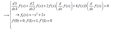
In this section, we consider the following differential equation and solve it by HPM, VIM and AGM semi-analytical approaches to analyze the precision of AGM.
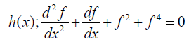 (23)
(23)
In this problem, the number of boundary conditions is one more than the order of the presented equation. The given equation should be derived so that the number of boundary conditions and the order of the differential equation will be equaled. Therefore, we will have:
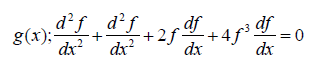 (24)
(24)
The corresponding boundary conditions are as below:
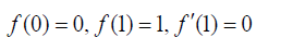 (25)
(25)
Applying HPM approach to the given equation
Considering Eq. 23 and 24, we construct the homotopy function as below:
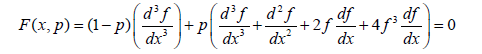 (26)
(26)
Assuming f(x) as a summation of a power series of parameter p, we will have:
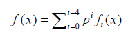 (27)
(27)
Substituting Eq. 27 into Eq. 26 and rearranging the answer by powers of p, the multipliers of each power are obtained. Solving the obtained answers according to the given boundary condition which is constant for all of them, the consecutive terms of HPM solution are gained:
 (28)
(28)
 (29)
(29)
 (30)
(30)
The answers of the next terms and the ultimate answer of Eq. 25 are presented in Appendix 1.
Applying VIM approach to the given equation
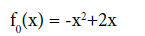
To apply the construction of the variational iteration method, we have to find the first sentence to start the loop.
By considering the linear sentence with maximum power of derivative  which is also the multiplier of power p0 in HPM method) and applying the corresponding boundary conditions, f0(x) can be found.
 (31)
(31)
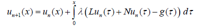
Based on the structure of VIM method, we construct the following formulation:
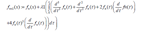 (32)
(32)
Considering an adequate Lagrange multiplier and setting n from 0 to 3, four terms of f(x) are calculated, the last cycle of this answer is known as the ultimate solution of the given equation.
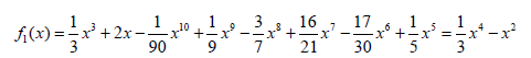 (33)
(33)
The answers of the next terms and the ultimate answer of Eq. 25 are presented in Appendix 2.
Applying AGM approach to the given equation
We first consider the given equation in the form below:
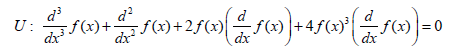 (34)
(34)
As it was discussed in the previous section, the answer of the differential equation is considered as a finite series of polynomials with constant coefficients:
 (35)
(35)
The aforementioned unknown coefficients are capable of being computed by applying the boundary conditions.
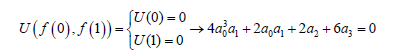
a) Applying the boundary conditions on Eq. 36:
 (36)
(36)
 (37)
(37)
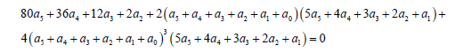
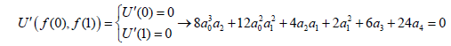
b) Applying the boundary conditions on the main differential Eq. 35 and its derivatives:
 (38)
(38)
 (39)
(39)
 (40)
(40)
 (41)
(41)
 (42)
(42)
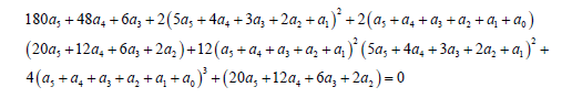
By solving a set of algebraic equations, six unknown coefficients are computed according to the existing six equations. By entering the values of the coefficients, the ultimate answer of AGM method is obtained.
Analogy between the methods is shown in Tables 4-6; Figures 4-15.
| x | f(x)-Maximum |Error| | ||
|---|---|---|---|
| HPM | VIM | AGM | |
| 0 | 0 | 0 | 0 |
| 0.1 | 1.24E-06 | 0.008563701 | 0.006869775 |
| 0.2 | 2.40E-06 | 0.016167488 | 0.011108978 |
| 0.3 | 2.97E-06 | 0.022796445 | 0.012703915 |
| 0.4 | 2.90E-06 | 0.028347035 | 0.012160051 |
| 0.5 | 2.38E-06 | 0.032627251 | 0.009832712 |
| 0.6 | 1.65E-06 | 0.035382979 | 0.006761654 |
| 0.7 | 9.31E-07 | 0.036353306 | 0.00318062 |
| 0.8 | 3.86E-07 | 0.035339905 | 0.000427369 |
| 0.9 | 8.31E-08 | 0.032258935 | 6.72E-05 |
| 1 | 4.00E-09 | 0.027139019 | 0 |
Table 4: Comparing the obtained charts by HPM, VIM and AGM for their f(x)-errors in accordance to the numerical approach.
| x | f‘(x) | |||
|---|---|---|---|---|
| HPM | VIM | AGM | Numerical | |
| 0 | 1.909404547 | 2 | 2.0025 | 1.909413569 |
| 0.1 | 1.727633922 | 1.808441316 | 1.7894 | 1.727647369 |
| 0.2 | 1.556743091 | 1.628011282 | 1.5901 | 1.556752052 |
| 0.3 | 1.389328156 | 1.450478213 | 1.3971 | 1.389330476 |
| 0.4 | 1.218431025 | 1.267967474 | 1.2034 | 1.218427709 |
| 0.5 | 1.03817714 | 1.0738019 | 1.0077 | 1.03817046 |
| 0.6 | 0.844968441 | 0.863996832 | 0.80784 | 0.844960853 |
| 0.7 | 0.638698783 | 0.638722634 | 0.6042 | 0.638692269 |
| 0.8 | 0.423436239 | 0.402993554 | 0.3987 | 0.423431972 |
| 0.9 | 0.207100456 | 0.165978303 | 0.19825 | 0.20709865 |
| 1 | -0.000000009 | -0.061143663 | 0.0077515 | 0 |
Table 5: Comparing the obtained charts by HPM, VIM, AGM and the numerical approach for f ‘(x).
| x | F’(x)-Maximum |Error| | ||
|---|---|---|---|
| HPM | VIM | AGM | |
| 0.1 | 9.02E-06 | 0.090586431 | 0.093086431 |
| 0.2 | 1.34E-05 | 0.080793947 | 0.061752631 |
| 0.3 | 8.96E-06 | 0.07125923 | 0.033347948 |
| 0.4 | 2.32E-06 | 0.061147737 | 0.007769524 |
| 0.5 | 3.32E-06 | 0.049539765 | 0.015027709 |
| 0.6 | 6.68E-06 | 0.03563144 | 0.03047046 |
| 0.7 | 7.59E-06 | 0.01903598 | 0.037120853 |
| 0.8 | 6.51E-06 | 3.04E-50 | 0.034492269 |
| 0.9 | 4.27E-06 | 0.020438418 | 0.024731972 |
| 1 | 1.81E-06 | 0.041120346 | 0.00884865 |
Table 6: Comparing the obtained charts by HPM, VIM and AGM for their f’(x)-errors in accordance to the numerical approach.

Figure 4: Comparison of HPM and the numerical method for f(x).

Figure 5: Comparison of VIM and the numerical method for f(x).

Figure 6: Comparison of AGM and the numerical method for f(x).

Figure 7: Comparison of HPM, VIM, AGM and the numerical method for f(x).

Figure 8: Comparison of HPM and the numerical method for f’(x).

Figure 9: Comparison of VIM and the numerical method for f’(x).

Figure 10: Comparison of AGM and the numerical method for f’(x).

Figure 11: Comparison of HPM, VIM, AGM and the numerical method for f’(x).

Figure 12: Comparison of HPM, VIM and AGM approaches for their f(x)- maximum errors.

Figure 13: Comparison of HPM, VIM and AGM approaches for their f(x)- maximum errors percent.

Figure 14: Comparison of HPM, VIM and AGM approaches for their f’(x)- maximum errors.

Figure 15: Comparison of HPM, VIM and AGM approaches for their f’(x)- maximum errors percent.
Conclusion
In this paper, we have successfully developed semi-analytical methods HPM, VIM & AGM to compute the given equation. We have utilized the Maple Package for our calculations. AGM & HPM methods were the most precise methods in this matter, so that they can be applied to the numerous questions arising in the fields of science and engineering day in day out [20-26].
Appendix 1
Description of the HPM approach: To elucidate on, consider the following equation:
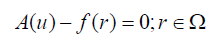 (43)
(43)
The boundary conditions are:
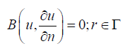 (44)
(44)
A: General differential operator, B: Boundary operator, f(r): Known analytical function
Γ : Boundary of the domain Ω
The operator A consists of linear and nonlinear parts, so the Eq. 1 can be rewritten in the form below [3,5]:
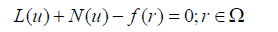 (45)
(45)
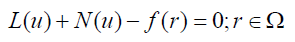
L: Linear part, N: Nonlinear part
The introduced structure of homotopy perturbation method is as below:
 (46)
(46)
While,
 (47)
(47)
p∈[0,1]: An embedding parameter, u0: First approximation satisfying the boundary condition
If the equation (4) be rewritten as a power series in p as below:
 (48)
(48)
The best approximation of the solution is considered as below:
 (49)
(49)
| x | f(x) | |||
|---|---|---|---|---|
| HPM | VIM | AGM | Numerical | |
| 0 | 0 | 0 | 0 | 0 |
| 0.1 | 0.181728983 | 0.190293926 | 0.1886 | 0.181730225 |
| 0.2 | 0.34588862 | 0.36205851 | 0.357 | 0.345891022 |
| 0.3 | 0.493193118 | 0.515992529 | 0.5059 | 0.493196085 |
| 0.4 | 0.623637046 | 0.651986985 | 0.6358 | 0.623639949 |
| 0.5 | 0.736564905 | 0.769194539 | 0.7464 | 0.736567288 |
| 0.6 | 0.830836697 | 0.866221325 | 0.8376 | 0.830838346 |
| 0.7 | 0.905118449 | 0.941472686 | 0.9083 | 0.90511938 |
| 0.8 | 0.958272246 | 0.993612536 | 0.9587 | 0.958272631 |
| 0.9 | 0.989767158 | 1.022026176 | 0.9897 | 0.989767241 |
| 1 | 1.000000004 | 1.027139019 | 1 | 1 |
Table 3: Comparing the obtained charts by HPM, VIM, AGM and the numerical approach for f(x).
Answer terms of the HPM approach to the Problem 2:
 (50)
(50)
 (51)
(51)
 (52)
(52)
Appendix 2
Description of the VIM approach: To clarify, note the equation below:
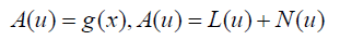 (53)
(53)
Where L & N represent the linear and nonlinear parts of the general differential operator A. g(x) is the inhomogeneous term of the equation. The introduced structure of the VIM method is as below [3]:
 (54)
(54)
λ is the general Lagrange multiplier which can be obtained by disparate ways including variational theory, Laplace method and etc. the subscript n represents the nth approximation of the solution, The appellation of  is justified by the fact that
 . The ultimate solution is given as:
 (55)
(55)
Answer terms of the VIM approach of Problem 2:
f3(x), f3(x); too many sentences.
References
- Ganji DD, Languri EM (2010) Mathematical methods in nonlinear heat transfer Book.
- Domairry G, Fazeli M (2009) Homotopy analysis method to determine the fin efficiency of convective straight fins with temperature-dependent thermal conductivity. Communications in Nonlinear Science and Numerical Simulation 14: 489-499.
- Ghafoori S, Motevalli M, Nejad MG, Shakeri F, Ganji DD,et al. (2011) Efficiency of differential transformation method for nonlinear oscillation: Comparison with HPM and VIM. Current Applied Physics 11: 965-971.
- Mehdipour I, Ganji DD, Mozaffari M (2010) Application of the energy balance method to nonlinear vibrating equations. CurrApplPhys 10: 104-112.
- Ganji DD, Ganji SS, Karimpour S, Ganji ZZ (2010) Numerical study of homotopy-perturbation method applied to Burgers equation in fluid. Numerical Methods for Partial Differential Equations 26: 917-930.
- Joneidi AA, Ganji DD, Babaelahi M (2009) Differential transformation method to determine fin efficiency of convective straight fins with temperature dependent thermal conductivity. International Communications in Heat and Mass Transfer 36: 757-762.
- Kern DQ, Kraus AD (1972) Extended surface heat transfer. McGraw-Hill, New York.
- Kraus AD, Aziz A, Welty J (2002) Extended surface heat transfer. John Wiley & Sons.
- Arslanturk C (2005) A decomposition method for fin efficiency of convective straight fins with temperature-dependent thermal conductivity. International Communications in Heat and Mass Transfer 32: 831-841.
- Zubair SM, Al-Garni AZ, Nizami JS (1996) The optimal dimensions of circular fins with variable profile and temperature-dependent thermal conductivity. International Journal of Heat and Mass Transfer 39: 3431-3439.
- Aziz A, Huq SE (1975) Perturbation solution for convecting fin with variable thermal conductivity. Journal of Heat Transfer 97: 300-301.
- Hatami M, Hasanpour A, Ganji DD (2013) Heat transfer study through porous fins (Si 3 N 4 and AL) with temperature-dependent heat generation. Energy Conversion and Management 74: 9-16.
- Ganji DD, Dogonchi AS (2014) Analytical investigation of convective heat transfer of a longitudinal fin with temperature-dependent thermal conductivity, heat transfer coefficient and heat generation. Int J PhysSci 9: 466-474.
- Hatami M, Ganji DD (2014) Natural convection of sodium alginate (SA) non-Newtonian nanofluid flow between two vertical flat plates by analytical and numerical methods. Case Studies in Thermal Engineering 2: 14-22.
- Dogonchi AS, Ganji DD (2016) Convection–radiation heat transfer study of moving fin with temperature-dependent thermal conductivity, heat transfer coefficient and heat generation. ApplThermEng 103: 705-712.
- Chol SUS (1995) Enhancing thermal conductivity of fluids with nanoparticles. ASME-Publications-Fed 231: 99-106.
- Jalili M, Baktash E, Ganji DD (2008) Application of He's homotopy-perturbation method to strongly nonlinear coupled systems. Int J Phys: Conference Series 96: 012078.
- Ahmadi AR, Zahmatkesh A, Hatami M, Ganji DD (2014) A comprehensive analysis of the flow and heat transfer for a nanofluid over an unsteady stretching flat plate. Powder Technology 258: 125-133.
- Aziz A, Benzies JY (1976) Application of perturbation techniques to heat-transfer problems with variable thermal properties. International Journal of Heat and Mass Transfer 19: 271-276.
- He JH (1999) Homotopy perturbation technique. Computer Methods in Applied Mechanics and Engineering 178:257-262.
- He JH, Wu XH (2006) Construction of solitary solution and compacton-like solution by variational iteration method. Chaos, Solitons& Fractals 29: 108-113.
- Barari A, Poor AT, Jorjani A, Mirgolbabaei H (2010) Analysis of diffusion problems using homotopy perturbation and variational iteration methods.Int J Res Rev ApplSci 14: 1101-1109.
- Mirgolbabaee H, Ganji DD, Ledari ST (2015) Heat transfer analysis of a fin with temperature-dependent thermal conductivity and heat transfer coefficient. New Trends in Mathematical Sciences 3: 55-69.
- Akbari MR, Ganji DD, Nimafar M, Ahmadi AR (2014) Significant progress in solution of nonlinear equations at displacement of structure and heat transfer extended surface by new AGM approach. Frontiers of Mechanical Engineering 9: 390-401.
- Meresht NB, Ganji DD (2016) Solving Nonlinear Differential Equation Arising in Dynamical Systems by AGM. International Journal of Applied and Computational Mathematics 1-17.
- Rostami A, Akbari M, Ganji D, Heydari S (2014) Investigating Jeffery-Hamel flow with high magnetic field and nanoparticle by HPM and AGM. Open Engineering 4: 357-370.
Relevant Topics
- Advanced Photovoiltoic Cells
- Advanced Photovoiltoic Panels
- Advanced Photovoiltoic Systems
- Advanced Photovoiltoic Technologies
- Alternative Energy
- Biomass Energy
- Coal Energy
- Energy Management
- Environmental Policy
- Green Energy
- Hydro Electric Energy
- Hydrogen Energy
- Hydropower Energy
- Photovoltoics
- Renewable Energy and Research
- Renewable Geothermal Energy
Recommended Journals
Article Tools
Article Usage
- Total views: 11837
- [From(publication date):
December-2016 - Aug 29, 2025] - Breakdown by view type
- HTML page views : 10830
- PDF downloads : 1007