Analytical and Numerical Method in the Free Convection Flow of Pure Water Non-Newtonian Nano fluid between Two Parallel Perpendicular Flat Plates
Received: 28-Aug-2016 / Accepted Date: 23-Sep-2016 / Published Date: 27-Sep-2016
Abstract
In this research, free convection of a non-Newtonian silver-water nanofluid between two infinite parallel perpendicular flat plates is investigated. The Maxwell Garnetts (MG) nanofluid model is used in this work. The basic partial differential equations are reduced to the ordinary differential equations which are solved analytically using Homotopy Perturbation Method (HPM). The impact of various physical parameters such as nanoparticle volume fraction (φ), dimensionless non-Newtonian viscosity (δ) and Eckert number (Ec) on the velocity and dimensionless temperature profiles is studied. The comparison of the results of HPM, Akbari-Ganji’s Method (AGM), Collocation Method (CM), the fourth-order Runge-Kutta numerical Method (NUM) and FlexPDE software results shows excellent complying in solving this problem. Also, this research shows that AGM and HPM are powerful methods to solve non-linear differential equations, such as the problem raised in this research.
Keywords: Free convection; Non-Newtonian; Nanofluid; Homotopy Perturbation Method; Akbari-Ganji’s method; Collocation method; FlexPDE software
19017Introduction
In fluid mechanics, we study the particles’ behavior at any point within the range of different physical conditions. Mathematical models are used to describe physical phenomena in fluid mechanics for a variety of fluids such as Newtonian and non-Newtonian fluids. More engineering problems, especially some of the heat transfer equations are non-linear. For this reason, resolving these difficult problems has been a controversial issue for mathematicians, physicists and engineers. Some equations are solved by numerical solutions; some are solved using different analytical methods. Methods that can be introduced to examine the non-linear problems such as the Differential Transform Method (DTM) [1-2], Least Square Method (LSM) [3-4], Akbari- Ganji’s Method (AGM) [5-8], Hamiltonian Approach [9], Variational Iteration Method (VIM) [10], and Adomian’s Decomposition Method (ADM) [11], many methods are not considered in this study because of brevity. One of the semi-analytical methods which does not need small parameters is the Homotopy Perturbation Method (HPM). The homotopy perturbation method, proposed first by He in 1998 and was further developed and improved by He [12]. This method in most cases provides fast convergence to solve series. Usually, due to the small number of trial and error, leads to the achievement of highprecision solutions. This new method is applied in a lot of researches in engineering sciences [13-17]. Heat transfer by free convection frequently occurs in many physical problems and engineering applications such as geothermal systems, heat exchangers, chemical catalytic reactors, fiber and granular insulation, packed beds, petroleum reservoirs and nuclear waste repositories [18-21]. In view of its importance, the flow of Newtonian and non-Newtonian fluids through two infinite parallel perpendicular flat plates has been examined by a large number of researchers. The natural convection problem between vertical flat plates for a certain class of non-Newtonian fluids has been carried out by Bruce and Na [22]. Other laminar natural convection problems involving heat transfer have been also studied by Ziabakhsh and Domairry [23]. Rajagopal and Na [24] presented an analysis for the natural convection in non-Newtonian fluid flow between two parallel plates. Yoshino et al. [25] presented a new numerical method for incompressible non-Newtonian fluid flows based on the lattice Boltzmann method (LBM). Pawar et al. [26] carried out an experimental study on isothermal steady state and non-isothermal unsteady state conditions in helical coils for Newtonian and non-Newtonian fluids. Also, numerous models and methods have been proposed by different authors to study convective flows of nanofluids and we mention here the papers written by Khan and Pop [27] Vajravelu et al. [28] and Yacob et al. [29]. The main aim of this work is to present the effects of nanoparticle volume fraction, dimensionless non-Newtonian viscosity and Eckert number on velocity profiles and temperature profiles in the flow of nanofluids between two infinite parallel perpendicular flat plates. The Maxwell–Garnetts (MG) nanofluid model [30] is used in this work. The reduced ordinary differential equations are solved analytically using HPM. The comparison of the results of HPM, Akbari-Ganji’s Method (AGM), Collocation Method (CM), the fourth-order Runge-Kutta numerical Method (NUM) and FlexPDE software results shows excellent complying in solving this non-linear problem.
Description of the problem
The schematic theme of the problem is shown in Figure 1. This figure includes two parallel plates, perpendicular to each other, in which there is a non-Newtonian fluid flowing due to the free convection between two parallel plates. The distance between the two plates is 2b. The walls at x= +b and x= -b are held at constant temperatures T2 and T1 , respectively, where T2>T1 . The difference between the two walls temperature makes the fluid near the wall, to rise at x=-b and fall at x=+b. The fluid is a water-based nanofluid containing silver. It is assumed that the source of fluid and nanoparticles are in thermal equilibrium, and no slip occurs between them. The thermo-physical properties of the nanofluid are listed in Table 1 [31].

Figure 1: Geometry of the considered problem.
| Material | Density (kg/m3) | Cp (J/kg.k) | K (w/m.k) | β× 10-5(k-1) |
|---|---|---|---|---|
| Pure water | 997.1 | 4179 | 0.613 | 21 |
| Silver | 10500 | 235 | 429 | 1.89 |
Table 1: Thermo-physical properties of water and nanoparticles [31].
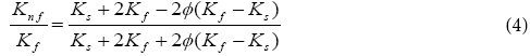
The effective density ( ρn f ), the effective dynamic viscosity ( μ n f ), the heat capacitance ( ρCp)n f and the thermal conductivity ( n f K ) of the nanofluid can be expressed as where (φ ) is the solid volume fraction.


Rajagopal [24] has demonstrated that by using the similarity variables:

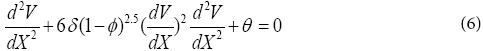
Under these assumptions and following the nanofluid model proposed by Maxwell–Garnetts (MG) model [30], the Navier-Stokes and energy equation can be reduced to the following pair of ordinary differential equations:
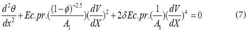
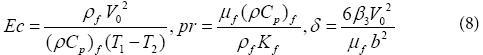
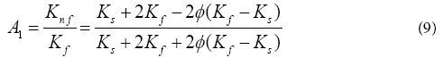
Where Prandtl number ( pr ), Eckert number ( Ec ), dimensionless non-Newtonian viscosity (δ ) and A1 have the following forms:
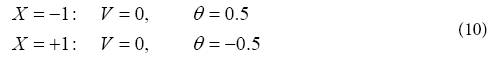
The appropriate boundary conditions are:
Mathematical Procedures
In this section three methods have been examined:
Homotopy perturbation method (hpm)
To explain the basic ideas of this method, we consider the following non-linear differential equation:
A(u)−f (r) = 0, r∈Ω (11)
With the boundary condition of:

Where A is a general differential operator, B a boundary operator, f (r) a known analytical function, (Γ ) is the boundary of the domain ( Ω ) and  denotes differentiation along the normal drawn outwards from ( Ω ).
A can be divided into two parts which are L and N, where L is linear part and N is non-linear part. Eq. (11) can therefore be rewritten as follows:
L(u) + N(u) − f (r) = 0 (13)
Homotopy perturbation structure is shown as follows:
H(ν , p)=L(ν )+L(u0 )+pL(u0 )+p(N(ν )−f (r)) = 0 (14)
Where,
ν (r, p) :Ω×[0,1]→R (15)
In Eq. (14), p∈ [0, 1] is an embedding parameter and u0 is the first approximation that satisfies the boundary condition. We can assume that the solution of Eq. (14) can be written as a power series in p , as following:
ν =ν+pν1+p2ν2 .............. (16)
and the best approximation for solution is:

Collocation method (cm)
Weighted residual method was first introduced by Ozisk [32] to solve the differential equation in heat transfer, Collocation and Galerkin method are analytical methods that are based on the weighted residual method.
Suppose a differential operator D, is applied on a function u to produce a function p
D(u(x)) = p(x) (18)
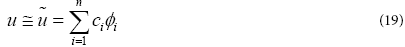
u is approximated by a function  , which is a linear combination of basic functions chosen from a linearly independent set. That is,
Now, when substituted into the differential operator, D, the result of the operations is not, in general, p(x) . Hence an error or residual will exist as

The main idea of the CM is to force the residual to zero in some average sense over the domain. That is:
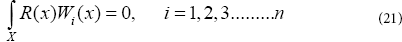
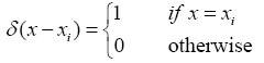
Where the number of weight functions Wi is exactly equal to the number of unknown constants ci in  function. The result is a set of n algebraic equations for the unknown constants ci. For collocation method, the weighting functions are taken from the family of Dirac functions in the domain. That is, Wix) =δ(x − xi) . The Dirac function has the property of:
Also, the residual function in Eq. (20) must be forced to be zero at specific points.
Akbari-Ganji’s Method (AGM)
Boundary conditions and initial conditions are required differential equation according to the physic of the problem. Therefore, we can solve every differential equation with any degrees. In order to comprehend the given method in this paper, two differential equations governing on engineering processes will be solved in this new manner. The nonlinear differential equation of p which is a function of u, the parameter u which is a function of x and their derivatives are considered as follows:
The non-linear differential equation p (which is a function of u ), the parameter u (which is a function of x ), and their derivatives are considered as follow:

Boundary conditions:
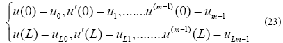
To solver the first differential equation, with respect to the boundary conditions in x = L in Eq. (23), the series of letters in the n th order with constant coefficients, which is the answer of the first differential equation, is considered as follows:

The boundary conditions are applied to the function as follows:
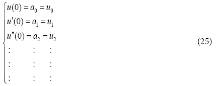
a) The application of the boundary conditions for the answer of differential Eq. (24) is in the form of
If x =0
And when x = L
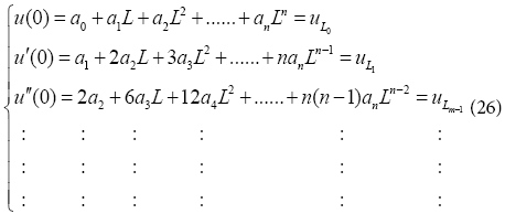
b) After substituting Eq. (26) into Eq. (22), the application of the boundary conditions on differential Eq. (22) is done according to the following procedure:
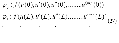
With regard to the choice of n; (n<m) sentences from Eq. (24) and in order to make a set of equations which is consisted of (n+1) equations and (n+1) unknowns, we confront with a number of additional unknowns which are indeed the same coefficients of Eq. (24). Therefore, to remove this problem, we should derive m times from Eq. (22) according to the additional unknowns in the afore-mentioned set differential equations and then this is the time to apply the boundary conditions of Eq. (23) on them.
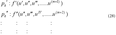
Application of the boundary conditions on the derivatives of the differential equation pk in Eq. (28) is done in the form of
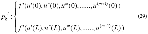
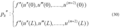
The ( n+1) equations can be made from Eq. (25) to Eq. (30) so that ( n+1) unknown coefficients of Eq. (24) for example, a0,a1,a2,a3 ........... an can be computed. The answer of the nonlinear differential Eq. (22) will be gained by determining coefficients of Eq. (24).
According to different works with AGM method and similar methods have been shown the AGM method is powerful method to solve non-linear problems. Because this method solves different variable such as power series, Sine and exp function at the same time and shows acceptable outcomes.
Application Of Described Methods In The Problem
Homotopy Perturbation Method (HPM)
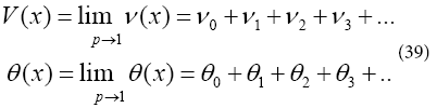
In this section, we will apply the HPM to non-linear ordinary differential Eqs. (6) and (7). According to the HPM, we construct a homotopy suppose the solution of Eqs. (6) and (7) has the form:
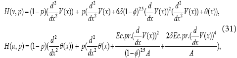
We consider V(x) and θ(x) as follows:
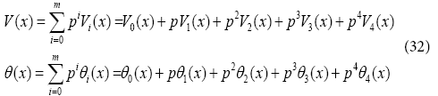
Substituting Eq. (32), into Eq. (31), and some simplification and rearranging on powers of P-terms, we have:
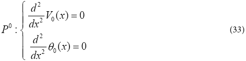
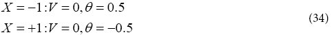
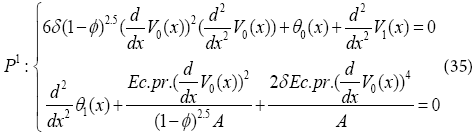
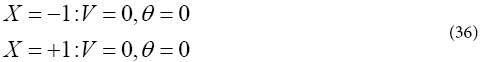
Solving Eqs. (33) and (35) with boundary conditions:
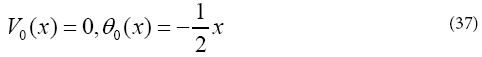
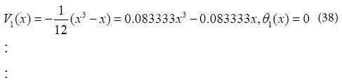
In the same manner, the rest of components were obtained by using the Maple package, that we obtain (32) parameters of it. According to HPM, we can conclude:
Collocation Method (CM)
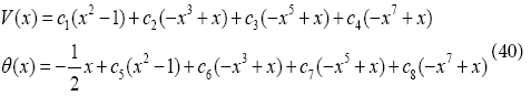
Since trial function must satisfy the boundary conditions in Eq. (10), so they will be considered as
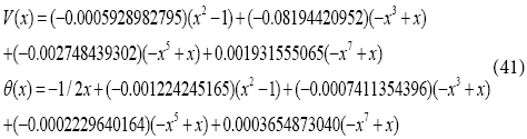
We select the collocation locations x=1/5 to 4/5 which are evenly spaced throughout the domain. Introducing these values into the residual Eq. (40). Thus we have eight algebraic equations for the determination of the eight unknown coefficients c1 to c8 . For example, Using collocation method with (Pr=0.5, Ec=0.5, φ =0.05, δ =0.5) V (x) and θ (x) are as follows:
Akbari-Ganji’s Method (AGM)
In order to solver the differential Eqs. (6) and (7), an answer function is considered as a finite series in the form of
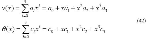
The given answer function has the constant coefficients c0 a to c3 a and 0 c to 3 c , which can easily be computed by applying the initial conditions from Eq. (10). It is notable that the more numbers of series sentences of Eq. (42), the more precise the answer, and the answer is tended to the exact solution [8]. For example, Using Akbari-Ganji’s Method with (Pr=1, Ec=0.1, φ=0.01, δ=0.2) a0 to a3 and c0 to c3 are as follows:
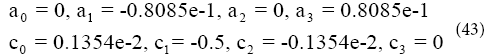
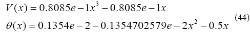
By substituting the constant coefficients from Eq. (43) into Eq. (42), the solution of the non-linear differential Eqs. (6) and (7) can be gained as
Solution whit flexpde software
In this study, we first introduce the FlexPDE software. FlexPDE software is simple modeling software based on finite element method for coding. This means that FlexPDE is a finite element method for coding. This means that FlexPDE converts written codes and partial differential equations to a finite element model. FlexPDE performs all necessary functions for solving partial differential equations as follows. Editing and preparation of texts, creating finite element network (grid), finite element solver organization for answers, adjusting the graphical output to delivered results. FlexPDE is a software that does not have a predetermined range of issues. The user is free for selection of equation. In addition, unlike commercial software, there is no doubt about what is the deal because the text fully describes the system of equations and the problem ranges. Another advantage of FlexPDE software is that equations or phrases can be added based on problem requirements. The problems that FlexPDE is capable of solving. Problems such as first or second order partial differential equations in (one, two or three) dimensional Descartes and geometry, one-dimensional spherical or cylindrical geometry, sustainable or transition system [33], linear or non-linear equations [34-35], eigen values problems, and several other issues are the problems that this simple software is able to solve. In this software, boundary conditions are applied when defining the problem boundaries. The primary types of boundary conditions are boundary are NATURAL, VALUE. NATURAL boundary conditions determine the value of a variable on the boundary of the domain NATURAL boundary conditions determine the amount of charge on the boundary of the domain Problem definition is divided into different parts in FlexPDE software. Determining variables, determining the geometry of the problem, determining material properties, determining the graphical output, applying boundary conditions include the parts of this simple software. The coding rules in this software are that they are not sensitive to lowercase or uppercase. A differentiation such as is shown like
 . All coordinate systems names are known valid such as second derivations like dxx (H) and differential functions such as Curl, Grad and Div. In this study, we compare the results of FlexPDE software with obtained results from HPM by writing FlexPDE software codes for Eqs. (6) and (7). For brevity, we evaluate only one case. For Figure 7, when (φ =0.03, δ=2, Ec =2, Pr=2), we have evaluated the velocity and temperature profiles. FlexPDE software codes for Eqs. (6) and (7) at (φ =0.03, δ=2, E =2, Pr=2) are given in Appendix A.
Results And Discussion
The comparison of the results of HPM with the results of the AGM, CM, Num and FlexPDE software results was conducted. Also, this research shows that AGM and HPM are powerful methods to solve non-linear differential equations.
Results of (HPM)

Figure 2: Effect of nanoparticle volume fraction (φ ) on (a) velocity profile (V(X)) and (b) temperature profile (θ(X)) when (Ec=1,δ=1, Pr=6.2).

Figure 3: Effect of dimensionless non- Newtonian viscosity (δ) on (a) velocity profile (V(X)) and (b) temperature profile (θ(X)) when (Ec=1, φ =0.05, Pr=6.2).

Figure 4: Effect of Eckert number (Ec) on (a) velocity profile (V(X)) and (b) temperature profile (θ(X)) when (δ=1, φ =0.05, Pr=6.2).
Comparison of numerical results with the results of (HPM)
Table 2
| V (x) | θ (x) | ||||
|---|---|---|---|---|---|
| x | Nu | HPM | Error | NuHPM | Error |
| -1 | 0.000000 | -1.00e-12 | 1.00e-12 | 0.500000 0.500000 | 0.000000 |
| -0.8 | 2.49e-02 | 0.024978 | -8.90e-05 | 0.404852 0.404687 | 0.000165 |
| -0.6 | 0.034361 | 0.034499 | -0.000138 | 0.307571 0.307541 | 2.94e-05 |
| -0.4 | 0.316000 | 0.031771 | -0.000171 | 0.210070 0.210225 | -0.000150 |
| -0.2 | 0.020505 | 0.020717 | -0.000212 | 0.112157 0.112397 | -0.000240 |
| 0.0 | 0.005037 | 0.005283 | -0.000246 | 0.013034 0.013246 | -0.000210 |
| 0.2 | -1.09e-02 | -1.07e-02 | -0.000254 | -8.77e-02 -8.76e-02 | -0.000140 |
| 0.4 | -2.35e-02 | -2.32e-02 | -0.000243 | -0.189907 -0.189774 | -0.000130 |
| 0.6 | -2.85e-02 | -2.83e-02 | -0.000234 | -0.292665 -0.292458 | -0.000210 |
| 0.8 | -2.19e-02 | -2.17e-02 | -0.000206 | -0.395570 -0.395312 | -0.00026 |
| 1 | 0.000000 | 1.00e-12 | -1.00e-12 | -0.500000 -0.500000 | 0.000000 |
Table 2: Comparison between Numerical results and HPM for V(x) and θ(x) when δ=1, Pr=6.2, ?=0.01, Ec=1.
Table 3
| V (x) | θ (x) | |||||
|---|---|---|---|---|---|---|
| x | Nu | HPM | Error | NuHPM | Error | |
| -1 | 0.000000 | 2.00e-11 | -2.00e-11 | 5.00e-01 0.500000 | 0.000000 | |
| -0.8 | 2.64e-02 | 0.026707 | -3.18e-04 | 0.412251 0.410966 | 1.28e-03 | |
| -0.6 | 0.037801 | 0.038229 | -4.28e-04 | 0.318437 0.317645 | 7.92e-04 | |
| -0.4 | 0.036652 | 0.037135 | -4.83e-04 | 0.223868 0.223923 | -5.43e-05 | |
| -0.2 | 0.026641 | 0.027227 | -5.87e-04 | 0.128579 0.129006 | -4.28e-04 | |
| 0.0 | 0.011684 | 0.012360 | -6.77e-04 | 0.030749 0.030992 | -2.43e-04 | |
| 0.2 | -4.42e-03 | -3.73e-03 | -6.90e-04 | -7.09e-02 -7.10e-02 | 9.29e-05 | |
| 0.4 | -1.78e-02 | -1.72e-02 | -6.59e-04 | -0.176022 -0.176076 | 5.45e-05 | |
| 0.6 | -2.44e-02 | -2.37e-02 | -6.60e-04 | -0.282871 -0.282354 | -5.16e-04 | |
| 0.8 | -1.96e-02 | -1.90e-02 | -6.13e-04 | -0.390062 -0.389033 | -1.03e-03 | |
| 1 | 0.000000 | 0.000000 | 0.000000 | 0.500000 -0.500000 | 0.000000 | |
Table 3: Comparison between Numerical results and HPM forV(x) andθ(x) when δ=2, Pr=6.2, ?=0.07, Ec=2.
Comparison of (CM) result with the result of (HPM)

Figure 5: Comparison of HPM and CM results when (Ec=0.5, =0.5, Pr=0.5, φ =0.05).
Comparison of (CM) results and (AGM) results with the results of (HPM)

Figure 6: Comparison of HPM, CM and AGM results when (Ec=0.1, =0.2, Pr=1, φ =0.01).
Comparison of FlexPDE software results with the results of (HPM)

Figure 7: Comparison of HPM, FlexPDE results when (Ec=2, =2, Pr=2, φ =0.03).
In the present study, free convection of a non-Newtonian nanofluid between two infinite parallel perpendicular flat plates has been investigated. These equations were solved analytically using the HPM, CM and AGM. In order to verify the accuracy of the present results, we have compared HPM results with numerical methods (the fourth-order Runge–Kutta method) and FlexPDE software. Comparison between HPM and numerical method are presented in Tables 1 and 2. For brevity, only two models, when (Pr=6.2, Ec=1, φ =0.01, δ=1) and (Pr=6.2, Ec=2, φ =0.07, δ=2), are discussed for velocity and temperature profiles. As seen in these Tables 1 and 2, for different values of x in the range of [-1, 1] error rate is very low, which indicates the good complying between the two methods. Also in this study the effect of various parameters such as nanoparticle volume fraction (φ ), dimensionless non- Newtonian viscosity (δ) and Eckert number (Ec) on velocity and dimensionless temperature profiles examined. Figures 2a and 2b show the effect of nanoparticle volume fraction (φ ) on the velocity and temperature profiles when (Ec=1, =1, Pr=6.2). According to the Figures 2a and 2b, by increasing nanoparticle volume fraction (φ ), the velocity and temperature profiles decline. Figures 3a and 3b, are shown the effect of dimensionless non-Newtonian viscosity (δ) on the velocity and temperature profiles, when (Ec=1, φ =0.05, Pr=6.2). The dimensionless non-Newtonian viscosity indicates the relative significance of the inertia effect compared to the viscous effect. According to the Figures 3a and 3b, by increasing dimensionless non-Newtonian viscosity (δ) velocity and temperature profiles decline. The effects of the Eckert number (Ec) on velocity profiles and temperature profiles when (δ=1, φ =0.05, Pr=6.2) are shown in Figures 4a and 4b, respectively. It is observed that due to the increasing velocity and temperature Eckert number (Ec) increases, when we ignore viscosity dissipation, the minimum values for the velocity and temperature are achieved. Figures 5a and 5b show the comparison between the results of HPM and Collocation method. In these Figures, we investigated the velocity and temperature profiles, when (Ec=0.5, δ=0.5, Pr=0.5, φ =0.05). The slight error between the Figures indicate the good complying between the two methods. Figures 6a and 6b show the comparison between the results of HPM, AGM and Collocation method. In these figures we examine one mode of (Ec=0.1, δ=0.2, Pr=1, φ =0.01) for velocity and temperature profiles. In accordance with the observed figures error is very low between the Figures, this means there is complying between the two methods.
Figures 7a and 7b show the comparison between the results of HPM and FlexPDE. In these figures we examine one mode of (Ec=2, δ=2, Pr=2, φ =0.03) for velocity and temperature profiles. The slight error in Figures indicate that HPM is a high accuracy method to solve these issues.
Conclusion
This paper has analyzed the phenomenon of free convection flow of a non-Newtonian nanofluid between two infinite parallel perpendicular flat plates using the HPM, AGM, CM and Num. The effects of the nanoparticle volume fraction (φ ), dimensionless non- Newtonian viscosity (δ) and Eckert number (Ec) on the velocity and dimensionless temperature profiles have been determined for a silver and water nanofluid with a Prandtl number of Pr=6.2. The results of this study indicate that increasing in nanoparticle volume fraction (φ ) leads to the decrease in the thickness of the boundary layer of the velocity and temperature. While increasing Eckert number (Ec) increases the velocity and temperature profiles. The results show that the HPM method hase excellent agreement with the fourth-order Runge-Kutta numerical Method (NUM) and FlexPDE software. As the most important result of this study it was observed that HPM and AGM are powerful methods to solve this kind of non-linear problems.
Appendix A
FlexPDE software codes:
Title ‘ Nanofluid between two parallel perpendicular flat plates’
Coordinates cartesian1 Variables V theta
Definitions Ks=42 Kf=0.613 phi=0.03 Pr=2 Ec=2 delta=2
A= (Ks+2*Kf-2*phi*(Kf-Ks))/(Ks+2*Kf+2*phi*(Kf-Ks))
Equations
V: dxx (V)+6*delta* (1-phi) ^2.5 * (dx (V)) ^2 * dxx (V)+theta=0
Theta: dxx (theta)+Ec*Pr* (((1-phi) ^ (-2.5))/A) *(dx (V)) ^2+(2) *delta*Ec*Pr*(1/A) *(dx (V)) ^4=0
Boundaries region 1 start (-1) point value (V)=0 point value (theta)=0.5
Line to (1) point value (theta)=(-0.5) point value (V)=0
Plots elevation (V) from (-1) to (1) elevation (theta) from (-1) to (1) tecplot (V) Tecplot (theta)
End
References
- Mosayebidorcheh S, Sheikholeslami M, Hatami M, Ganji DD (2016) Analysis of turbulent MHD Couettenanofluid flow and heat transfer using hybrid DTM–FDM. Particuology 26: 95-101.
- Sheikholeslami M, Ganji DD (2015) Nanofluid flow and heat transfer between parallel plates considering Brownian motion using DTM. Comput Meth ApplMechEng 283: 651–663.
- Hatami M, Hasanpour A, Ganji DD (2013) Heat transfer study through porous fins (Si 3 N 4 and AL) with temperature-dependent heat generation. Energy Conversion and Management 74: 9-16.
- Hatami M, Ganji DD (2014) Natural convection of sodium alginate (SA) non-Newtonian nanofluid flow between two vertical flat plates by analytical and numerical methods. Case Studies in Thermal Engineering 2: 14-22.
- Akbari MR, Ganji DD, Goltabar AR (2014) Dynamic Vibration Analysis for Non-linear Partial Differential Equation of the Beam-Columns with Shear Deformation and Rotary Inertia by AGM. Development and Applications of Oceanic Engineering 3: 22-31.
- Akbari MR, Ganji DD, Ahmadi AR, Kachapi SH (2014) Analyzing the nonlinear vibrational wave differential equation for the simplified model of Tower Cranes by Algebraic Method. Frontiers of Mechanical Engineering 9: 58-70.
- Akbari MR, Ganji DD, Majidian A, Ahmadi AR (2014) Solving nonlinear differential equations of Vanderpol, Rayleigh and Duffing by AGM. Frontiers of Mechanical Engineering 9: 177-190.
- Ahmadi A (2015) Nonlinear Dynamic in Engineering by Akbari-Ganji’s Method.Xlibris Corporation.
- Nianga JM, Recho N (2014) Hamiltonian approach to piezoelectric fracture. Procedia Materials Science 3: 318-324.
- Biazar J, Gholamin P, Hosseini K (2010) Variational iteration method for solving Fokker–Planck equation. J Franklin Inst 347: 1137-1147.
- Wu GC (2011) Adomian decomposition method for non-smooth initial value problems. Math Comput Model 54: 2104-2108.
- He JH (2004) Comparison of homotopy perturbation method and homotopy analysis method.Appl Math Comput 156: 527-539.
- Sheikholeslami M, Ashorynejad HR, Ganji DD, Kolahdooz A (2011) Investigation of Rotating MHD Viscous Flow and Heat Transfer between Stretching and Porous Surfaces Using Analytical Method. Mathematical Problems in Engineering pp: 17.
- Barari A, Ghotbi AR, Farrokhzad F, Ganji DD (2008) Variational iteration method and Homotopy-perturbation method for solving different types of wave equations. Journal of Applied Sciences 8: 120-126.
- Domairry D, Sheikholeslami M, Ashorynejad HR, Gorla RSR, Khani M (2011) Natural convection flow of a non-Newtonian nanofluid between two vertical flat plates. Journal of Nanoengineering and Nanosystems 225: 115-122.
- Ganji DD, Nezhad HRA, Hasanpour A (2011) Effect of variable viscosity and viscous dissipation on the Hagen-Poiseuille flow and entropy generation. Numerical Methods for Partial Differential Equations 27: 529-540.
- Jalaal M, Ganji DD, Ahmadi G (2010) Analytical investigation on acceleration motion of a vertically falling spherical particle in incompressible Newtonian media. Advanced Powder Technology 21: 298-304.
- Hatami M, Ganji DD (2013) Heat transfer and flow analysis for SA-TiO 2 non-Newtonian nanofluid passing through the porous media between two coaxial cylinders. Journal of Molecular Liquids 188: 155-161.
- Sheikholeslami M, Gorji-Bandpy M, Ganji DD (2013) Natural convection in a nanofluid filled concentric annulus between an outer square cylinder and an inner elliptic cylinder. Sci Iran Trans B: MechEng 20: 1241-1253.
- Sheikholeslami M, Gorji-Bandpy M, Domairry G (2013) Free convection of nanofluid filled enclosure using lattice Boltzmann method (LBM). Appl Math MechEng Ed 34: 833-846.
- Hatami M, Nouri R, Ganji DD (2013) Forced convection analysis for MHD Al 2 O 3–water nanofluid flow over a horizontal plate. Journal of Molecular Liquids 187: 294-301.
- Bruce RW, Na TY (1967) Natural convection flow of Powell–Eyring fluids between two vertical flat plates. ASME 67: 25.
- Ziabakhsh Z, Domairry G (2009) Analytic solution of natural convection flow of a non-Newtonian fluid between two vertical flat plates using homotopy analysis method. Commun Nonlinear SciNumerSimul 14: 1868-1880.
- Rajagopal KR, Na TY (1985) Natural convection flow of a non-Newtonian fluid between two vertical flat plates.ActaMech 54: 239-246.
- Yoshino M, Hotta Y, Hirozane T, Endo M (2007) A numerical method for incompressible non-Newtonian fluid flows based on the lattice Boltzmann method. J Non-Newton Fluid Mech 147: 69-78.
- Pawar SS, Sunnapwar VK (2013) Experimental studies on heat transfer to Newtonian and non-Newtonian fluids in helical coils with laminar and turbulent flow. Experimental Thermal and Fluid Science 44: 792-804.
- Khan WA, Pop I (2010) Boundary-layer flow of a nanofluid past a stretching sheet. Int J Heat Mass Transf 53: 2477-2483.
- Vajravelu K, Prasad KV, Lee J, Lee C, Pop I, et al. (2011) Convective heat transfer in the flow of viscous Ag-water and Cu-water nanofluids over a stretching surface. Int J Thermal Sci 50: 843-851.
- Yacob NA, Ishak A, Pop I, Vajravelu K (2011) Boundary layer flow past a stretching/shrinking surface beneath an external uniform shear flow with a convective surface boundary condition in a nanofluid. Nanoscale Res Lett 6: 314.
- Xuan Y, Roetzel W (2000) Conceptions for heat transfer correlation of nanofluids. Int J Heat Mass Transf 43: 3701-3707.
- Aminossadati SM, Ghasemi B (2009) Natural convection cooling of a localised heat source at the bottom of a nanofluid-filled enclosure.Eur J Mech B/Fluids 28: 630-640.
- Sheikholeslami M, Ganji DD (2014) Three dimensional heat and mass transfer in a rotating system using nanofluid. Powder Technology 253: 789-796.
- Sheikholeslami M, Ashorynejad HR, Domairry G, Hashim I (2012) Flow and heat transfer of Cu-water nanofluid between a stretching sheet and a porous surface in a rotating system. Journal of applied mathematics pp: 1-18.
- Sheikholeslami M, Hatami M, Ganji DD (2014) Nanofluid flow and heat transfer in a rotating system in the presence of a magnetic field. Journal of Molecular liquids 190: 112-120.
Citation: Gholinia M, Ganji DD, Poorfallah M, Gholinia S (2016) Analytical and Numerical Method in the Free Convection Flow of Pure Water Non-Newtonian Nano fluid between Two Parallel Perpendicular Flat Plates. Innov Ener Res 5: 142.
Copyright: ©2016 Gholinia M, et al. This is an open-access article distributed under the terms of the Creative Commons Attribution License, which permits unrestricted use, distribution, and reproduction in any medium, provided the original author and source are credited.
Select your language of interest to view the total content in your interested language
Share This Article
Recommended Journals
Open Access Journals
Article Usage
- Total views: 11047
- [From(publication date): 12-2016 - Aug 31, 2025]
- Breakdown by view type
- HTML page views: 10068
- PDF downloads: 979