Control of HIV/AIDS Infection System with Reverse Transcriptase Inhibitors Dosages Design via Robust Feedback Controller
Received: 14-Jul-2017 / Accepted Date: 08-Sep-2017 / Published Date: 12-Sep-2017 DOI: 10.4172/2090-4967.1000146
Abstract
Acquired Immune Deficiency Syndrome (AIDS) is a disease or continuum condition which is due to Human Immunodeficiency Virus (HIV) infection. One in five people are infected with HIV are not aware of the infection. Early detection of the infection helps the infected people to take medications to avoid future consequences and reduce the risk of transmitting the disease. Reverse transcriptase inhibitors (RTIs) were the first available drug and were considered a principal kind of medication available to treat HIV patients. These drugs are still successful, effective, and are considered to have imperative solutions for treating HIV when joined with different medications. Investigating effect of this branch of the drugs on HIV and model this interaction has a great of importance to control AIDS.
This need can be addressed by the control system engineering which uses control theory to estimate and design a system. Since Stability is the most significant requirement of the system, and a system of instability cannot be expected for a particular transient reaction or steady state error specification then objective which is needed to be achieved by working on this research is to design a stabilized model of a patient having AIDS. In this research feedback controllers, Root locus technique and Routh Hurwitz method have been adopted to design such an advanced transformative controller which robustly regulates RTIs infusion dosages considering the amount of HIV viruses in infected human body.
Keywords: AIDS; HIV; RTIs; Modelling; Control; Stabilized model; Feedback controller; Root locus technique; Routh Hurwitz method
Introduction
AIDS stands for Acquired Immune Deficiency Syndrome [1-4]. Letter “A” stands for “Acquired” which means that it is a condition obtained, implying that a man gets to be contaminated with it [5,6]. Letter I stands for “Immune” which means HIV influences a man's resistant framework, the part of the body that battles off germs, for example, microbes or infections [7,8]. Letter D stands for “Deficiency” which means that the resistant framework gets to be lacking and does not work legitimately [9,10]. Letter S stands for “Syndrome” which means a person with AIDS might encounter different sicknesses and diseases in light of a debilitated insusceptible framework [4,11] Feinberb and Moore proposed an AIDS model to know the influence of medicine or vaccines on the HIV virus [12]. The vast majority of these medications come as tablets or capsules [13]. The lab makes a figuring in light of aggregate white blood cells and the extent of cells that are CD4 [14]. On the other hand, if the CD4 count is lesser then 200 cells/mm3 this implies that the individual has diagnosed a stage 3 infection of AIDS [15].
Initially the discussion was regarding what can be done in order to control AIDS and what are techniques present today which can help an infected person to keep the level of the virus to a lower level [16,17]. The perspectives from the point of view of control theory which control systems are present to design the feedback system to control these viruses in an infected individual [18,19]. Next section of the research explains how the CD4 cells work and how they were developed and what can be done in order to control the infection and what factors determines the HIV life cycles and what is meant by the viral load count, how the lab tests are conducted on the bases of the CD4 count [20,21]. How can be a linear system and a non-linear framework distinguished [22]. Similarly, one of the important points covered in this section of the research enlightens on how the linearization works and how to determine the equilibrium points in a given framework [23].
Methodology
The state space representation of system can be expressed in state equation. The state variable is linearly self-determining and the choice affects the matrices. Transfer function is expressed as state space [24]. After the virus has be found out in the body and when the retroviral drug has been injected the system is altered. The system is modelled by linearizing resulting to the virus free system.
Next is analysing the technique to discover a state response of multivariable time changing systems. Systems are normally presented by an arrangement of differential equations via a state space model [25]. Usually, it is a thorough and difficult task to solve the time varying state space representation [24]. Representation of a time response requires the solving of the space dynamic by initial conditions. This requires the computing of the state transition matrix first. Laplace transforms equations to obtain efficiency and effectiveness of the drug that is used to fight against the virus.
Stability is the most vital requirement of the system, in this section; stability is discussed by applying Routh-Hurwitz method [26]. Routh- Hurwitz criterion is used to obtain a constant that will determine the stability of the system, which will give us an idea to use a suitable amount of drug to keep the spread of infection stable.
At the last root locus is used to design and analysis of the system. It helps in getting in knowing the details regarding the stability and the response system. We also discussed the different methods of sketching the root locus. In this chapter we focused on the gain adjustment. The gain modification is only done after the transient response is found out. The section is concluded by understanding positive feedback system and sketching the root locus of the mentioned system [27].
Feedback system
Control system engineering is a part of engineering which uses control theory to estimate and design a system [28]. There are four functions in the control theory i.e., measure, compare, compute and correct [29]. The open-loop control system framework uses an actuating device to control the procedure specifically without utilizing device [30]. The main reasons of using the block diagram rather than using other methods that block diagram analyse a simple control system in a way which cannot be analysed by the other methods because this method helps us in understanding the operation of the problem statement and how the control theory plays an important role in understanding the procedure of the given problem. Block diagram is a method which gives us the symbolic representation of complex signals making the problem easier so that it can be understood clearly it is a method which also helps to establish a relationship in between the subsystems. As by this method complicated equations which are representing the schematics can be avoided in other words this method helps an individual to understand the problem in the easiest way by avoiding all the complications. Block diagrams are normally utilized for larger amount, less point by point portrayals that are expected to clear up general ideas without the apprehension for the details of implementation [31].
The two drugs reverse transcriptase inhibitors (RTIs) and protease inhibitors (PIs) will be used as input variables for the feedback of the system. A “controller” which helps to decide that in which quantity these drugs must be injected in the body of an infected person because the combination of these drugs plays an important role in maintaining the level of the HIV viruses referred as the output for the feedback of the system. The block diagram of such a system has been shown in Figure 1.

Figure 1: Block diagram.
Linearization
Problem can be solved by using the method of linearization. In a control system framework if any non-linear systems are present at that point it becomes necessary that the system must be linearize before the transfer function of a system have to be determined.
The final type of non-linearity which is important to discuss is “backlash nonlinearity” which means when the input course is altered at that point the output becomes steady till the input surpasses a firm assessment (the backfire is dispensed with nonlinear control systems analysis [32].
The first step in this method is to perceive the non-linear part and compose the non-linear differential mathematical statement. In the next step we linearize the non-linear differential mathematical statement, and after that we take the Laplace transformation of the linearized differential mathematical statement, accepting zero as the starting condition. Lastly, we isolate input and as well the output variables which perform an important role in the forming of a transfer function [27].
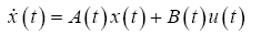
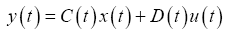
The transfer function is expressed in terms of state space. The general way of expressing the linear state equation of state space is [33]:
 (1)
(1)
 (2)
(2)
Where the variables have been defined as shown in Table 1.
| Variables | Abbreviation |
|---|---|
| X | state vector |
 |
derivative of the state vector with respect to time |
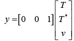
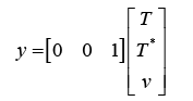
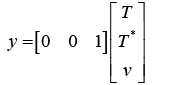
| Y | output vector |
| U | input or control vector |
| A | system matrix |
| B | input matrix |
| C | output matrix |
| D | feed forward matrix |
Table 1: Variables defined for the Equations 1 and 2.
The result is obtained by two steps firstly by the state variable response is obtained and then by substituting it to obtain the y (t). The method used mostly is matrix method where the vector values are reduced into scalar values and are assigned to the respective matrices. For selecting a state vector the minimum number of state variable should be chosen as the factor of the state vector, the number of state variable explains the state of the system and factors should be linearly independent.
Laplace transforms system
As elucidated in previous section that systems were demonstrated in state space, where the state-space representation comprised of a state comparison and an output mathematical statement. In this segment, we utilize the Laplace change to tackle the state mathematical statements for the state and yield vectors. The Laplace transform is a reliable method for resolving ordinary and partial differential equations.
As mentioned earlier, RTIs drug is used to fight against the infection. Our main objective here in this section is to find the efficiency of the drug, which is to find  . At the end, we will approximate a time the drug could take to show its highest possible effectiveness.
Laplace transforms solution of state equations as follows [27]:
Laplace transform of the input equation:
 (3)
(3)
Laplace transform of the output equation:
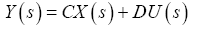 (4)
(4)
State space representation
We have seen in previous section that systems were demonstrated in state space, where the state-space representation comprised of a state comparison and an output mathematical statement. In this segment, we utilize the Laplace change to tackle the state mathematical statements for the state and yield vectors.
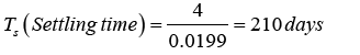
For the performance of the system, settling time formula of the first order system is used [27]. State space representation is a mathematical illustration of a system where the input and output of the transfer function including the state variable is represented by the first order differential equation [34]. The system could be formulated by utilization of Kronecker vector matrix structures [35,36]. The state variables are a subset and can depict the system state in a given time [27]. The order of the system is equivalent to the reduced denominator [29]. The general method of expressing the linear representation of state space is representing them as time invariant. As the system is dynamic the time invariant could be discrete or continuous [37,38]. In the course of the most recent decade, numerous effective hypotheses were created for first-order system definition of Stokes and Navier-Stokes equations. The first-order system presented in for Stokes comparisons included velocity, velocity flux, and pressure [39]. Equation of the Laplace is the most significant of all partial differential equations [40].
Routh-Hurwitz method
The objective of this section is to design a stable controller of the system. Stability is an important specification of the system. Routh- Hurwitz criterion is the method used to generate the information of stability by determining the number of poles [27]. The Routh-Hurwitz method involves two stages; producing Routh table and determining the Routh table to find out the number of poles in the planes and axis [27]. According to Routh- Hurwitz method, if all the poles are in the left-half plane then the system is stable. The system is unstable if any poles are in the right-half plane. The reason of being marginally stable is due to having undamped sinusoidal mode [41]. The graph gives us the idea regarding the zero as well as the poles of a transfer function of a dynamic system in a complex plane [42].
The characteristic equation illustrate the value of the gain, it estimates the behaviour of the system with changing values of the controller gain [29]. Controllability of a system is used to stabilize system by feedback or optimal control. Observability is a measure in which the present state can be decided on the fixed time interval using the output function [43].
Root locus
Root locus is a graphical technique which helps in inspecting the variety which happened in the roots of control system [27]. In the continuous transfer domain (CT) zeroes are the root of the polynomial of numerator and poles are for the denominator. The region of convergence (ROC) of a transfer function is a half-plane or vertical strip, either of which contains no poles [44]. In discrete time system the region of convergence contains no poles. The system has right sided impulse if the ROC moves away from the pole with progressive value other than infinite and then no poles are at infinity [45].
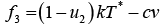
The steps for drawing a root locus are drawing the forward-loop poles and zeros and part of the locus that lies on the real axis then locating the centroid and sketching the asymptotes. Then by locating break point and estimating angles of arrival and departure. Calculating the imaginary axis crossing and then drawing the rest of the locus. By plotting the root locus it provides a detailed view of the stability of the closed loop controller. When two or more root loci converge initially and then diverges, that point is considered as break points. They occur in real as well as complex plane, but mostly real axis. The gain ‘K’ is calculated by dividing the product of the length between each pole to the point by the product of the length between each zero to the point.
Results And Discussion
The problem states that we have to design a block diagram which plays an important role in controlling the HIV viruses which are entering in the body of an infected individual. While constructing this block diagram we have to keep in mind the parameters for instance what will be the inputs and outputs. In this case we know that the two drugs reverse transcriptase inhibitors (RTIs) and protease inhibitors (PIs) will be used as input variables for our design of the block diagram as how much of these drugs are dispensed in the body of the infected person. As we need to consider the feedback of the system while designing the system so it is becoming clear that for this case we will be using a closed-loop system framework.
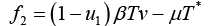
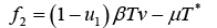
By the problem statement it is becoming clear that we have to apply linearization approach in order to find out the transfer function. We also know that the model present in the problem statement resembles the non-linear system framework which signifies the equations. Now the important thing which needs to be determined in the (a) part of the problem is to find out which equations are having the linear and nonlinear characteristics. The first two equations are non-linear because of the  products on the right side [27]:
 (5)
(5)
 (6)
(6)
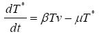
Now in the (b) part of this problem we have to determine the two equilibrium points present in the system in order to simplify the situation [27]:
To find the equilibrium let
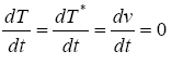 (7)
(7)
Leading to:
 (8)
(8)
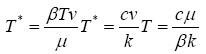
Substituting the latter into the first equation after some algebraic manipulations we get that
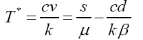 (9)
(9)
In this section we need to achieve the state space representation by linearizing the equation with equilibrium condition limiting to zero.
 (10)
(10)
 (11)
(11)
 (12)
(12)
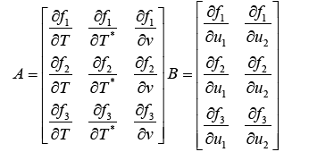 (13)
(13)
Then just by direct substitution:
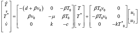 (14)
(14)
 (15)
(15)
 (16)
(16)
 (17)
(17)
Where the variables have been defined as shown in Table 2
| Symbol/Abbreviation | Units |
|---|---|
| t (Time) | days |
| d (Death of uninfected T cells) | 0.02 day |
| k (Rate of free viruses produced per Infected T cell) | 100 counts/cells |
| s (Source term for uninfected T cells | 10 mm3/day |
| β (Infectivity rate of free virus particles) | 2.4 × 10⁻⁵mm3/day |
| c (Death rate of viruses) | 2.4 day |
| μ (Death rate of infected T cells) | 0.24 day |
Table 2: Typical parameter values for HIV/AIDs model (27).
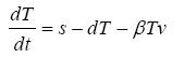
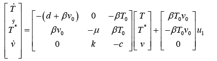
After the substitution of parameter values,
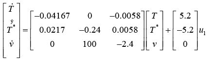 (18)
(18)
 (19)
(19)
Thus,
By making an assumption that RTIs are 100% effective, we will approximate the time RTIs would take to show maximum effectiveness.
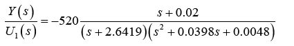
The transfers function of the human immunodeficiency virus infection calculated in the previous chapter:
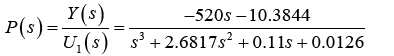 (20)
(20)
Considering K as a constant and the objective is to find a range of K by using Routh-Hurwitz method to determine that the system is closed loop stable.
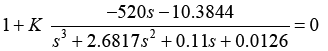 (21)
(21)
Therefore for system’s stability:
 (22)
(22)
And
 (23)
(23)
The transfer function is linearized where the virus levels are controlled by the RTIs. Then to plot the root locus for all value of the gain greater than zero, initially for the open loop transfer function where the transfer function is greater equal to the gain; we need to show that which system is stable for the open loop transfer function for value of gain above zero.
(a) The open loop transfer function is
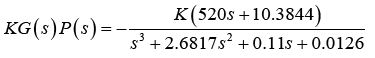 (24)
(24)
To obtain the breakaway points let
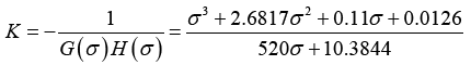 (25)
(25)
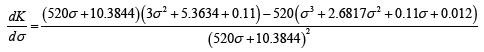 (26)
(26)
The value of K at σ=0.0446 is 6.82 × 10⁻⁴. We have already found this result in the previous problem. That the system is closed loop stable for k<2.04 × 10⁻⁴. The root locus sketch has been illustrated in Figure 2.

Figure 2: Positive feedback system.
Now for negative feedback system,
The value of K at σ=-1.33 is 0.0033 and value of K at σ=- 0.0879 is 6.5 × 10⁻⁴
We use Routh-Hurwitz to show that the system is closed loop stable for all >0. The characteristic equation is:
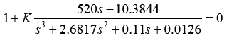 (27)
(27)
The Routh Array has been calculated as shown in Table 3.
| Symbols | Equations | |
|---|---|---|
| S3 | 1 | 0.11+520K |
| S2 | 2.6817 | |
| S | 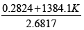 |
-- |
| S0 | 0.0126+10.3844K | -- |
Table 3: Routh Table (27).
The denominator of the transfer function is considered since we are keen in the poles of the system. At first, the columns are filled with powers of s from the most elevated power of the denominator of the closed-loop transfer function to s°. The remaining entries are filled according to the Routh- Hurwitz method as follows. Every section is a negative determinant of entries in the past two lines and determinant is divided by the entry which is present in the primary column specifically over the computed line. The left-hand segment of the determinant is dependably the main section of the past two lines, and the right-hand segment is the components of the segment above and to right side. The table is said to be complete when all the rows are calculated down to s°. It can easily be verified that all the entries in the first column are positive for all k>0 The root locus sketch has been shown in Figure 3.

Figure 3: Negative feedback system.
In the negative feedback system, we could estimate that the number of branches is equal to the number of the poles which is obtained from the graph. The poles are symmetrical about the real axis. From the graph we could find out that for the root locus begins at poles and ends at the zeroes. The angle of the complex pole is used to obtain the damping ratio. The distance from the pole to the origin is referred as the natural frequency. As we have found out the damping ratio, the lines in the graph represent the damping lines; it helps to estimate the settling time, damped oscillation frequency and the overshoot. As the settling time decrease the damping ratio increase, likewise the rise time and peak time also decreases with the increase in the damping ratio. Taking overshoot percentage into criteria, the value reduces when the damping ratio increases. The compensator design is a modification of the root locus when the present situation where it is not possible to obtain the desired transient distinctiveness, so we alter it by adding zeroes or poles. Increasing in damping ratio is approximately referred as dropping of angle of the asymptotes.
Conclusion And Future Work
Every year, millions of people die due to AIDs worldwide. It is estimated that 1.2 million people died due to AIDs related illness in the year of 2014 [46]. The death rate clearly makes the AIDs one of the most dangerous life taking disease of mankind. Since there is no cure for AIDs, controlling and monitor of AIDs can be a useful tool for the reduction of the spread of the virus.
In this paper, how the spread of the infection can be controlled is discussed, analysed and elaborated by the implementation of mathematical equations. Medication by means of drugs is used throughout our research as an input of the system. In section one; we obtained a clear feedback block diagram of the system after drugs used as input. Transfer function of the disease in found in the second section. Since the infection is non-linear, linearization of the system to obtain the space representation is done in section three. The effectiveness and the time to show maximum effectiveness are the core requirement of a successful drug. Based on assumptions, efficiency and time are calculated in section four. Stabilizing of the virus depending on the amount of the drugs required are analysed and discussed in section five. In the final section, graphical generation of the feedback systems are shown and explained. This research paper was only constrained to computer simulation. Future researchers can emphasis on development and employment of the testing apparatus for the simulations accomplished in this paper.
There is significant amount of probability regarding more work which can be done in the light of this research. In this research parametric study was constructed mainly but for the future many possibilities are present which can be done.
Artificial intelligence techniques such as Artificial Neural Networks (ANN) [47-49], Ring Probabilistic Logic Neuron [50,51], Fuzzy logic [52] and Genetic algorithm [53] are important algorithms which can be taken in account in order to perform the modelling of AIDS as future work.
Acknowledgment
The author(s) declare(s) that there is no conflict of interest regarding the publication of this paper.
References
- Sepkowitz KA (2001) AIDS-the first 20 years. Mass Medical Soc. New England J Med 344: 1764-1772.
- Alexander K, Mirjam K, Klaus K (2010) Modern infectious disease epidemiology. Concepts, methods, mathematical models, Springer Publications, Germany.
- Wilhelm K (2008) Encyclopedia of public health. Springer Publications, Germany.
- Friedl GH, Harris C, Butkus-Small C, Shine D, Moll B, et al. (1985) Intravenous drug abusers and the acquired immunodeficiency syndrome (AIDS):Demographic, drug use, and needle-sharing patterns: JAMA 145: 1413-1417.
- Friedman N, Deborah, Kaye KS, Stout JE, McGarry SA, et al. (2002) Health care-associated bloodstream infections in adults: A reason to change the accepted definition of community-acquired infections: Am Coll Physicians 137: 791-797.
- Wang CY, Wang JJG (1989)Rapid immunoagglutination test for presence of HIV in body fluids. US 4879211 A.
- Carrington M, O'Brien SJ (2003) The influence of HLA genotype on AIDS*. Ann Rev Med 54: 535-551.
- Connie M, Donald L, George M (2014) Textbook of diagnostic microbiology: Elsevier Health Sciences, UK.
- Budka H (1986) Multinucleated giant cells in brain: A hallmark of the acquired immune deficiency syndrome AIDS 69: 253-258.
- James MH, Stanley EA (1988) Using mathematical models to understand the AIDS epidemic. Math Biosci 90: 415-473.
- Shattock RJ, Doms RW (2002) AIDS models: Microbicides could Learn from vaccines. Nature Med 8: 425.
- Gostin LO, Curran WJ, Clark ME (1986) Case against compulsory casefinding in controlling AIDS-testing, screening and reporting, The: HeinOnline, Am JL Med 12.
- An SF, GrovesM, Giometto B, Beckett AA, Scaravilli F (1999) Detection and localisation of HIV-1 DNA and RNA in fixed adult AIDS brain by polymerase chain reaction/in situ hybridisation technique. Acta Neuropathol 98: 481-487.
- Ian KC, Xiaohua X (2005) Can HIV/AIDS be controlled? Applying control engineering concepts outside traditional fields, Control Systems. IEEE 25: 80-83.
- Granich RM, Gilks CF, Dye C, De Cock KM, Williams BG (2009) Universal voluntary HIV testing with immediate antiretroviral therapy as a strategy for elimination of HIV transmission: A mathematical model. The Lancet 373: 48-57.
- Dalgleish AG, Beverley PC, Clapham PR, Crawford DH, Greaves MF, et al. (1984) The CD4 (T4) antigen is an essential component of the receptor for the AIDS retrovirus. Nature 312: 763-767.              Â
- Perelson AS, Kirschner DE, De Boer R (1993) Dynamics of HIV infection of CD4+ T cells. Math Biosci 114: 81-125.
- Xia X, Moog CH (2003) Identifiability of nonlinear systems with application to HIV/AIDS models: IEEE, Automatic Control, IEEE Transactions on 48: 330-336
- Saadat H (1993) Computational aids in control systems using MATLAB. McGraw-Hill, NY, USA.
- Woolford A (2001) Tainted space: Representation of injection drug-use and HIV/AIDS in Vancouver's downtown eastside. BC Studies 129: 27-50.
- Paul JVB, Cajo JFTB (1999) Principal response curves: Analysis of time-dependent multivariate responses of biological community to stress. Wiley Online Library, UK. 18: 138-148.
- HillDJ, Moylan PJ (1977) Stability results for nonlinear feedback systems. Automatica 13: 377-382,
- Norman SN (2011) Control system engineering: John Wiley & Sons Inc, USA.
- Karl JA, Richard M (2010) Feedback systems: An introduction for scientists and engineers: Priceton University Press, NY, USA.
- Richard CD, Robert HB (2001) Introduction to control systems. Modern Control Systems (9th edn), : Prentice Hall International, NJ, USA.
- John PH (2012) Computer Architecture and Organization. McGraw Hill Publishing Company, USA. pp. 89-92.
- William LB (1974) Modern control theory. New Jersey: Prentice Hall International Inc, Universityof Nevada, Las Vegas, USA.
- Gopal M (2003) Digital control and state variable methods: Conventional and neural-fuzzy control systems. New Delhi, India. Tata McGraw-Hill Publishing Company Limited.
- Vasilyev AS, Ushakov AV (2015) Modeling of dynamic systems with modulation by means of Kronecker vector-matrix representation. SciTech J Inf Technol Mech Opt15: 839-848.
- Feng L (2007)Â Robust control design: An optimal control approach. West Sussex : John Wiley & Sons Ltd, USA.
- Kozák S, Huba M (2004) Control Systems Design 2003, Oxford Elsevier Ltd, UK.
- Karl J, Bjorn W (2011) Computer-controlled systems theory and design. (3rd edn): Dover Publications, Inc, USA.
- Kim SD, Chang OL, Thomas AM, Stephen FMC, Oliver R (2006) First-order system least-squares for the oseen equations. Wiley Online Library, USA. 31: 1785–1799
- Renardy M, Rogers RC (2004) An introduction to partial differential equations. (2nd edn), Springer, Germany.
- Clark RN (1992)The Routh- Hurwitz Stability Criterion. IEEE12: 119-120.
- Dimitris GM, Vinay KI(2011) Applied digital signal processing: Theory and practice. Cambridge University Press, UK.
- Podofillini L, Sudret B, Stojadinovic B, Zio E, Kröger W (2015) Safety and reliability of complex engineered systems: ESREL.
- Ronald LA, Duncan M (2004) Signal analysis: Time, frequency, scale, and structure: John Wiley & Sons Inc, NJ, USA.
- Alan VO, Ronald WS, Buck JR (2010) Discrete-time signal processing: Prentice Hall, USA.
- http://www.unaids.org/en/resources/documents/2015/AIDS_by_the_numbers_2015
- Aydin A, Navid S (2009) Mathematical modeling of dermal wound healing's remodeling phase: A finite element solution, Singapore.
- Aydin A, Kambiz GO (2010) Modeling of forced dermal wound healing using intelligent techniques: IEEE.
- Aydin A (2013) Introducing neural networks as a computational intelligent technique: Trans Tech Publications, Switzerland. 464: 369-374.
- Aydin A (2017) Introducing a novel hybrid artificial intelligence algorithm to optimize network of industrial applications in modern manufacturing.Complexity 18.
- Aydin A, Ali VB, Majid H ( 2016) Optimizing radio frequency identification network planning through ring probabilistic logic neurons: Sage Publications, USA.
- Kambiz GO, Aydin A (2010) Optimizing fuzzy logic controller for diabetes type I by genetic algorithm: Transtech 2.
- Aydin A, Ali A (2014) Introducing genetic algorithm as an intelligent optimization technique: Transtech 568: 793-797.
Citation: Azizi A (2017) Control of HIV/AIDS Infection System with Reverse Transcriptase Inhibitors Dosages Design via Robust Feedback Controller. Biosens J 6: 146. DOI: 10.4172/2090-4967.1000146
Copyright: ©2017 Azizi A. This is an open-access article distributed under the terms of the Creative Commons Attribution License, which permits unrestricted use, distribution, and reproduction in any medium, provided the original author and source are credited.
Select your language of interest to view the total content in your interested language
Share This Article
Recommended Journals
Open Access Journals
Article Tools
Article Usage
- Total views: 21804
- [From(publication date): 0-2017 - Dec 17, 2025]
- Breakdown by view type
- HTML page views: 20478
- PDF downloads: 1326