Biosensors Journal
Open Access

Dermal wounds are deep skin wounds that should be well-taken care of since this type of wounds might damage the organ integrity after losing tissue. In dermal wound repair, certain interacting phases occur after the damage is done to the skin. These events are: Inflammation, tissue formation, angiogenesis, tissue contraction and tissue remodeling [1].

The interaction of the cells with the ECM (Extracellular Matrix) is of great importance to all these phases. After the formation of blood clot during the inflammation, white blood cells attack the wound site by migrating through the ECM. Fibroblasts also migrate into the wounded area afterwards and start replacing the clot with collagen. Migrated fibroblasts tend to biochemically alter the ECM by degrading the fibrin and producing collagen [2].

As the new tissue is being created, endothelial cells migrate into the region and tend to form a new vasculature called angiogenesis [3]. The best result would be a healed wound possessing new tissue totally similar to that surrounding it. This, however, is not always the case. The architecture upon which the new tissue is created is different from the original and is usually less functional. The regenerated and different tissue is called a scar.

What makes a scar different from the original skin is an altered structure and composition in the dermis. Normally scars possess less blood vessels that are responsible for providing denser connective tissue which is less elastic with blood. The orientation of fibrous matrix seems to be the most considerable difference between the normal tissue and scar tissue. In rodents, a reticular collagen pattern can be found in normal tissues, whereas scar tissues form large parallel bundles at approximately right angles to the basement membrane [4]. Scar tissue associated to human is the same, having more collagen density, bigger fibers and more alignment in comparison to normal tissue, though the alignment is parallel to the skin [5].

A different ratio of collagen types and a lack of hair follicles and sweat glands are other structural differences between scars and normal tissues. In this research our focus will be on the cell density. The ultimate objective of this study is to remove scars. Inside a wound is being constantly remodeled during the preliminary stages of healing process, and for months or years the scar remains visible and mechanically noticeable. Wound healing is obviously an important issue to take care of. For instance, among dermal wounds, serious burns are very common causing sustain thermal injuries in more than 2 million Americans annually. However, there are a whole lot of other consequences to wound healing. It is proven that there is a relation between the scar formation and fibro plastic diseases such as Dupuytren’s contracture [6] and also the appearance of stretch marks during pregnancy [7] which is an example of sustained tissue deformation after stretching.

Now after introduction, in next section we analyze how the wound healing process actually works then on section 3, an appropriate mathematical model for dermal wound healing with fucusing on remodeling phase is intruduced, next in section 4 we try to model wound healing process with artificial neural networks, and at the end in section 5 we try to controll the wound healing procidure with disigning neural networks controller (NNC), and have thorough analysis on the results and conclusion in chapters 6 and 7 respectivly.

The concept of a “Wound” involves the gross macroscopic or subliminal microscopic damage to the anatomical and functional integrity of live tissues [8,9]. The diverse clinical symptoms of injury vary from noticeable cutaneous injuries [10] to scenarios involving subtle metabolic microangiopathies [11]. Irrespective of the specific etiology and external manifestation, the restoration of the original status of the wounded tissue is a result of a similar sequence of events that follows the injury. The healing process of the anatomical integrity of full-thickness cutaneous wounds in adult mammals tends to be a highly orchestrated phenomenon which demands harmonized interactions of various cellular and extracellular elements.

The repair progresses through several overlapping phases which include inflammation, proliferation and remodeling (Figure 1) [9,10]. The final outcome and the entire process are pretty sensitive to the alteration of any of the interrelated elements involved in healing [12,13]. Some examples are defective healing response secondary to stress-induces immunomodulation [12,14].

Figure 1: Cutaneous wound repair phases: There are 3 phases for a wound healing process: inflammation (early and late), proliferation and remodeling. These processes are plotted along the abscissa as a logarithmic function of time. A considerable overlap can be observed in terms of these phases. There are early and late inflammations denoting neutrophil-rich and mononuclear cellrich infiltrates, respectively [17].

The inflammatory phase provides cellular and extracellular elements with the scaffolding needed for the proliferation and migration to the wound site. Proliferation phase proceeds through proliferative activity of various cellular elements, e.g. endothelial cells, fibroblasts, epithelial cells, etc. However, the restoration of normal functional and anatomical properties of the wounded tissue is the final purpose of the healing response. Remodeling of the newly formed tissue at the site on which injurious stimuli occur is necessary for adaptation of the functional and mechanical properties of the wound site and adjacent unwounded tissues.

The remodeling procedure step is of the highest importance which determines the final fate of the regenerated tissue. While normal remodeling leads to the development of original tissue structure and anatomy, abnormal remodeling causes serious consequences; among which are scarring of the wounded area and non-healing wounds. Thus, it is very important to determine both the nature of how the affecter signals should be controlled and the mechanism underlying their effect.

There is a highly sophisticated sequence of overlapping events to the healing process of a dermal skin wound. The initial one is called coagulation cascade [15] in which fibrinogen, a soluble protein in the plasma, is changed to fibrin that polymerizes to generate blood clot. This clot tends to stop bleeding and can dry and create a scab that ultimately covers the wound; there is also a provisional matrix formed by the clot which acts as a scaffold for the attack of various cell types. After 24 to 48 hours [15,16] the wound is infiltrated by fibroblasts which dissolve the fibrin clot sand replace it with a collagen matrix. The composition of the ECM is altered within a period of months by dermal fibroblasts as the final phase of wound healing [17].

Remodeling phase of wound healing process

Remodeling phase deals with shift in the composition of the extracellular matrix fibers and cells. To illustrate better what happens in remodeling phase (Figure 2). Collagen type III which is a higher modulus of elasticity in comparison to type I is deposited during proliferation phase. There can be seen a gradual change from type III to type I, that has a lower modulus of elasticity, during the procedure. Extracellular enzymes collectively called matrix metalloproteinase (MMPs) tend to degrade collagen part III. However, tissue inhibitors of metalloproteinase (TIMPs) are secreted so that a level of control over these enzymes can be implied. Thus, a relatively controlled degradation of type III collagen is the result of the counterbalancing activity of TIMPs over MMPs. Surprisingly, as illustrated in the diagram; collagen degradation products (CDPs) encourage the proliferative activity of fibroblasts. However, this is a different scenario in that the secretion of collagen type I instead of type III is involved. This results in a dynamic physical status because of the change of the collagen type III/type I ratio. The modulation of the effect of external and internal forces that exist over wound region is the result of the ratio of collagen type III/ type I which can be regarded as a definition of the physical attributes of the wound site. There is a concurrence of reorganization of the collagen fibers and the alteration of their direction. These fibers, during second deposition, are arranged in a parallel fashion with the forces active over the wound region. It is known that collagen fibers demonstrate piezoelectric properties and therefore create electrical currents when affected by mechanical strain.

Figure 2: Remodeling phase.

The main stimulatory growth factor acting over fibroblasts is transforming growth factor-beta which promotes the secretion of collagen fibers. Nevertheless, there is a synergistic interaction between the created piezoelectricity and TGF-beta. What they have in common is that both tend to increase the metabolic activity of fibroblasts in a synergistic fashion. Therefore, piezoelectricity has two targets: fibroblasts and TGF-beta itself and its receptors. On the other hand, the differentiation of myofibroblasts is induced by TGF-beta. Myofibroblasts have contractile properties and make a contribution towards wound contraction. However, the effect of these cells is exerted through collagen fibers. That is the reason why the pattern of strain generated by myofibroblasts is affected by the orientation of collagen fiber. In fact, the main sources of internal strain are myofibroblasts.

The external strain is the result of certain sources like kinesthetic movements of neighboring tissues. The orientation of collagen fibers and afterwards the generation of piezoelectricity are affected by both internal and external strains. The change in the deep geometry of the wound region as well as the stress-relaxation and stress-concentration areas is the result of wound contraction- not epithelialization. Thus, the modulation of wound geometry is worthy of our consideration.

Though ECM-fibroblast interactions are well-researched, this area is poorly known [18]. One reason is that all interactions have not been discovered, the main reason, though, is that the involved processes interact in a very complicated manner with nonlinear feedback. Such complex feedback mechanisms can be easily addressed by mathematical modeling. There are certain assumptions taken into account when formulating the following models. These assumptions are a few wellknown interactions which are briefly summarized.

Firstly, the orientation of the matrix tends to direct fibroblast movement. This is a phenomenon called “Contact Guidance” [19- 21]. Secondly, the speed of the fibroblasts is affected by the ECM. It is proven that the matrix composition has an effect on the mobility of fibroblasts that migrate more easily on fibronectin gels than on collagen gels [22]. Thirdly, the production of different proteins by the fibroblasts is highly sensitive to the composition of the ECM [23,24]. Fourth, a plethora of growth factors and cytokines that alter fibroblast behavior can be found in the ECM in the wound region. Finally, fibroblasts tend to organize the thin collagen fibrils into the fibrous structure noticeable in the dermis [19].

Two of these interactions are of great importance to our models and require more explanation. Firstly, he “Contact Guidance” has been proven directly when fibroblasts put on oriented collagen gels attack the gels in the direction of orientation [25]. More proof to this behavior can be observed when fibroblasts migrate along fibronectin fibrils [26]. The next key interaction is associated to the way collagen is produced by fibroblasts and the complex process by which the collagen polymerizes to form a fibrous network of matrix [27]. The fibroblasts release procollagen molecules through secretory vesicles. Deep, narrow recesses in the fibroblasts’ cell surface are created by the fusion of these vesicles with the cell membrane. The collagen fibrils are formed in these recesses. There is a theory that these deep recesses provide the fibroblasts with the control over the micro-environment in which the collagen fibrils are forming and therefore control over the structure of the resulting collagen matrix [28].

The collagen matrix is itself considered to be an important frame work used by migrating fibroblasts as scaffolding to crawl on. Therefore, as the fibroblasts affect the orientation of the matrix, the matrix orientation influences the directed movement of the fibroblasts.

Extracellular matrix remodeling in soft connective tissues is induced by both biochemical and biomechanical stimuli [13,29]. The morphology and (mechanical) behavior of the stimulated tissue is greatly affected by the remodeling process [30]. Mechanically induced extracellular matrix remodeling is an important role player in tissue engineering of load-bearing structures, such as cartilage [31] and heart valves [32].

A mathematical model is necessary to have a deeper understanding of the processes of tissue remodeling. The model should include both the causes and consequences of the remodeling processes. It can easily be observed that this model acts as a useful tool for tissue engineering applications to optimize the mechanical conditioning protocol and to acquire the desired tissue integrity; efficient protocols cannot be designed unless an understanding of the tissue’s response to mechanical stimuli is gained. These protocols may be of great assistance in manipulating the process of remodeling toward the desired result.

The model of dermal wound healing that we use here is a model of fibroblasts cells [33]. In this research attempted to represent the cells (n) as independent entities owing to the scales involved.

A typical mobile fibroblast can have different lengths ranging values of the order 100 mm, and the diameters of the collagen fibers are of the order 1 mm [28,34]. In addition, what makes the independent representation more realistic is that normal dermal tissue is relatively sparsely populated with cells. It should also be noted that during wound healing more cells are employed to the region.

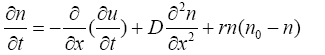
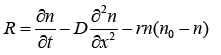
The cell conservation equation is:

(3.1)

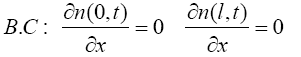
Boundary conditions (B.C) of (1) are:

(3.2)

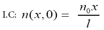
Initial condition (I.C) of (1) is:

(3.3)

The cell conservation consists of the usual terms, namely, the cell density n with uninjured steady state value n₀, diffusion with coefficient D, convection along with the extra cellular matrix (ECM) at velocity ∂u/∂t together with inhibition of cell mitosis for high cell density which is qualitatively again modeled by a logistic type growth curve rn (n₀−n), where r is the mitotic rate. The velocity, ∂u/∂t, is an approximation to the convection velocity. In remodeling phase this velocity is ignorable, here we assume ∂u/∂t=0.01 is wound length and -l/2<x<l/2. Parameters values are r=1, D=0.1 [35].

Uninjured steady state values n₀ depend on person is variable, here we assume n₀=1 (number/ml or number/mm²), also we assume wound shape as a circle (R=l/2). We use finite element method to solve (3.1).

Finite element method

As well as changes in time, the variable(s) being modeled may be dependent on position (space). When modeling the accumulation of fibroblast, for example, it may be important to specify where there is a buildup rather than just calculating the total amount present. This results in partial differential equations where the dependent variable Φ depends on a number of spatial variables, as well as time (Φ[x,t] or Φ[x,y,t] in 2D and 3D, respectively).

To solve such equations numerically it is necessary to discretize in both space and time. The standard method for this is the finite difference method, which splits up each spatial direction using a fixed step size. This produced a mesh (often referred to as a grid in 1D or 2D) with joints termed “nodes.” The data value of Φ (x,y,t) at the node (x_i, y_j) at time t_k is given by Φ_i,j,k. By again replacing derivatives (here usually in both time and space) with differences, the system of differential equations is reduced to a set of algebraic equations in Φ_i,j,k, which may be solved computationally. The issue of what boundary conditions are imposed on the space being considered (or what initial conditions are given) is not discussed here, except to say that this will obviously influence the choice of numerical method to be used. Although the above systems deal well with a large variety of models, it is sometimes important to represent more complex objects, such as skin stretched over bone. These differences in physical geometry are important when considering areas such as the ankle, where venous ulcers occur. Finite element methods mark out the surface of an object by covering it with nodes (reference points), which are then joined together (usually with 3 neighbors) to provide a (triangular) mesh covering the entire surface. This can be extended to higher dimensions to consider not only surfaces but also spaces, necessary in fluid dynamics for example.

To solve (3.1) as told before we consider the wound shape as a circle with R=l/2, at first, we suppose R as an interval named an element (e) (Figure 3) and then we will extend R to more elements.

Figure 3: Wound shape.

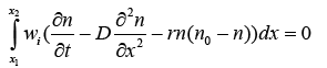
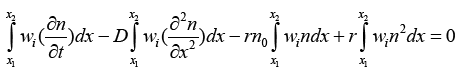
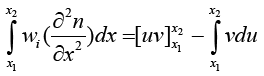
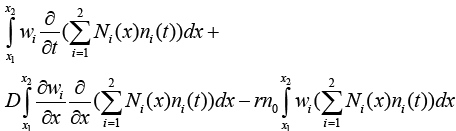
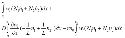
Now we write weak form integration for this element as seen below:

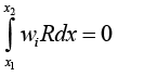(3.4)

w_i is defined as below:

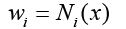(3.5)

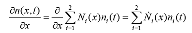
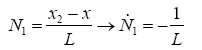
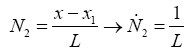
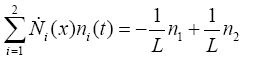
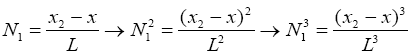
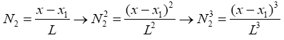
Which i is node's number and N_i(x) is named shape function. As seen below we use linear functions to define shape functions (Figures 4 and 5):

Figure 4: Dividing R to 3 equal intervals.

Figure 5: Linear shape functions of an element.

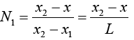(3.6)

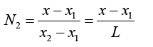(3.7)

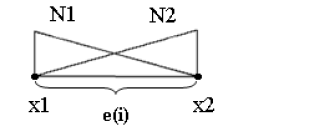
Linear shape functions of an element

It is important to note that in some locations, there may be significantly more happening than in others. On a mesh used to represent an object surface, each node represents a point where the solution will be calculated. The solution for the remaining area is then estimated by averaging the surrounding nodes.

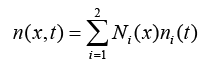
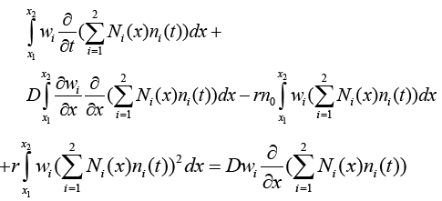
R is defined as below:

(3.8)

With substituting (3.8) in (3.4) we have:

(3.9)

So:

(3.10)

Solution of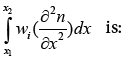

(3.11)

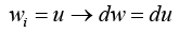(3.12)

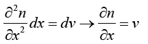(3.13)

So (3.11) become:

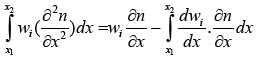(3.14)

With replacing (3.14) in (3.10) we have:

(3.15)

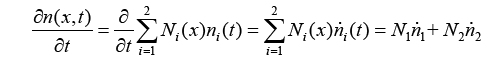
In the other hand we know:

(3.16)

(3.17)

So with replacing (3.5) and (3.17) in (3.15):

(3.18)

(3.19)

(3.20)

(3.21)

(3.22)

With replacing (3.21) and (3.22) in (3.20):

(3.23)

With replacing (3.19) and (3.23) in (3.18):

(3.24)

(3.25)

With replacing (3.5) in (3.24):

(3.26)

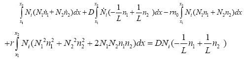
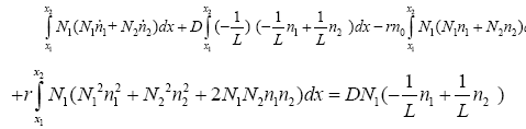
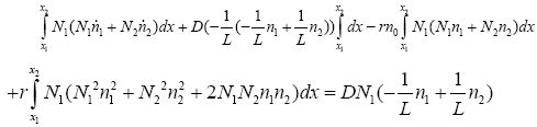
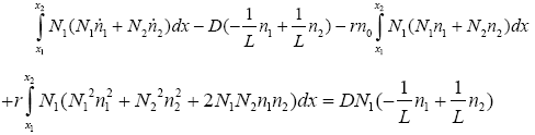
Now we rewrite (3.25) first for N₁ and next for N₂:

With replacing N₁ in 3:25:

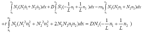(3.27)

(3.28)

(3.29)

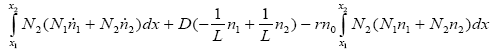
With replacing N2 in (3.25):

(3.30)

With replacing (3.22) in (3.30):

(3.31)

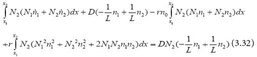
From (3.29) and (3.32):

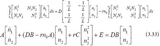
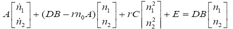
We restate (3.33) as seen below:

(3.34)

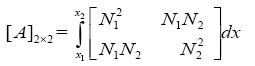
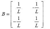
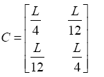
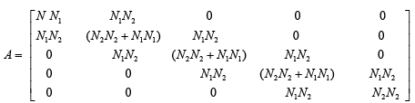
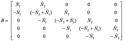
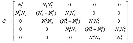
Which in (3.34) matrixes A, B, C and E are defined as shown below:

(3.35)

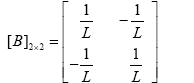(3.36)

(3.37)

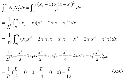
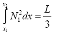
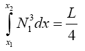
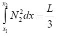
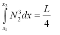
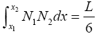
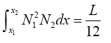
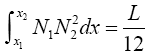
To compute elements of matrixes A, B, C and E we act as below:

(3.39)

(3.40)

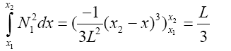
(3.41)

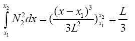
(3.42)

(3.43)

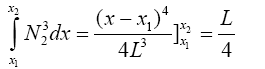
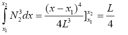(3.44)

(3.45)

(3.46)

(3.47)

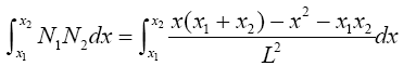
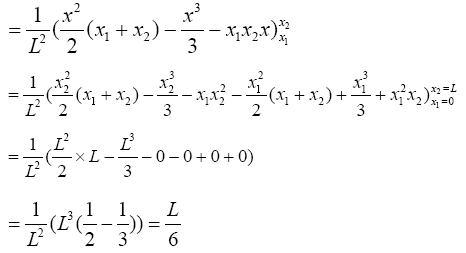(3.48)

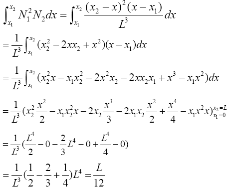(3.49)

So parameters values are:

(3.51)

(3.52)

(3.53)

(3.54)

(3.55)

(3.56)

(3.57)

With substituting (3.51)-(3.57) in (3.35)-(3.37):

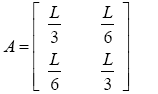(3.58)

(3.59)

(3.60)

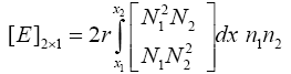
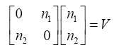
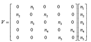
Finding matrix E is more complex than the others, to find matrix E we restate this matrix as shown below:

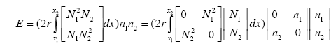(3.61)

(3.62)

With replacing (57) and (62) in (61):

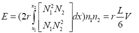(3.63)

With replacing (63) in (34):

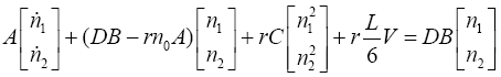(3.64)

(3.65)

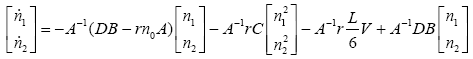
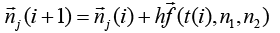
Now with knowing matrixes A, B, C and V we can solve (3.65). To solve this nonlinear equation numerically, Euler method is used as seen below:

(3.66)

With replacing (3.66) in (3.65):

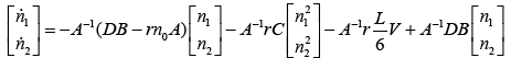(3.67)

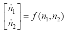
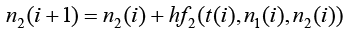
(3.68)

j is number of nodes j = 1,2 and i is time j = 0,1,2,……..

(3.69)

(3.70)

The results for R=10 mm along 1600 days which wound healing process is completely done are reported in Figure 6.

Figure 6: Cell conservation along R for two nodes. ( 0 ≤ x ≤ R ).

Now we can increase node number by dividing wound length to more elements. In this moment, we do not need to compute matrixes A, B, C and V again because they can be computed by assembling in base of one element's solution as seen in next two examples:

• Example 1

We divide wound length to 4 equal intervals (elements) made from 5 nodes.

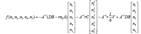(3.71)

(3.72)

j is number of nodes j = 1, 2, 3, 4, 5 and i is time i = 0, 1, 2, 0…….

Matrixes A, B, C

(3.73)

(3.74)

(3.75)

(3.76)

With substitute matrix parameters from equations (3.51)-(3.57) matrixes A, B and C are computed as below:

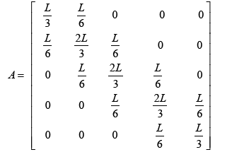(3.77)

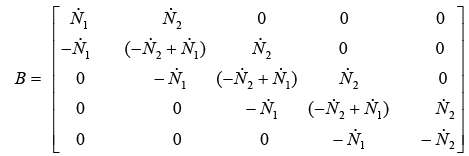(3.78)

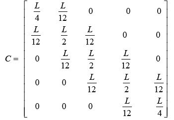(3.79)

So the results are:

• Example 2

We divide wound length to 9 equal intervals (elements) made from 10 nodes.

(3.80)

(3.81)

j is number of nodes j =1, 2,3,...,10 and i is time i = 0,1,2,.....

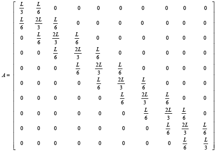
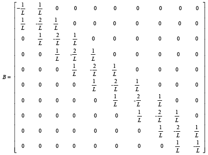
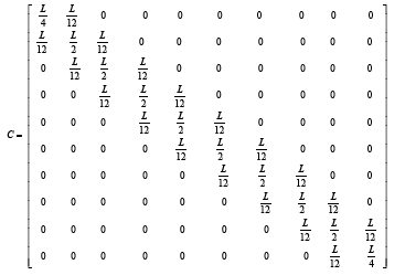
Matrixes A, B, C, and V are written as shown below:

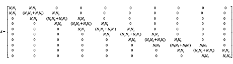(3.82)

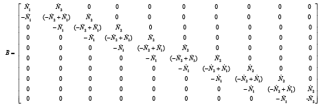
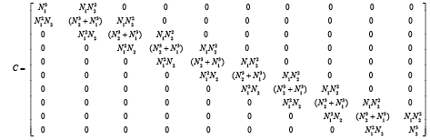
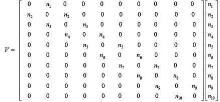
With substitution matrix parameters from equations (3.51)-(3.57) matrixes A, B and C are computed as below: 0 0 0 0 0 0

(3.86)

(3.87)

(3.88)

We compute cell concentration in dermal wound healing process with 2, 5 and 10 nodes. With comparing matrixes, A, B, C and V in different node number assumptions, it is seen that there is a logical rule in assembling each of these matrixes, and they can be extended to more nodes by writing an appropriate software coding program (Figures 7-9). For this purpose we use MATLAB software.

Figure 7: Cell conservation along R for 5 nodes. ( 0 ≤ x ≤ R ).

Figure 8: Cell conservation along R for 10 nodes. ( 0 ≤ x ≤ R ).

Figure 9: Cell conservation along R for 100 nodes. ( 0≤x≤R ).

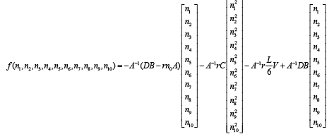
The extended form of cell conservation equation's solution is as seen below:

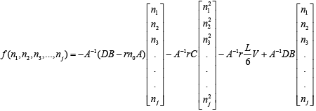(3.89)

(3.90)

j is number of nodes j =1,2,3,... and i is time i = 0,1,2,.....

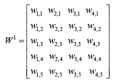
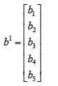
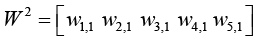
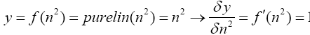
To model wound healing process, we use neural networks' architecture with a two-layer network; each layer has its own weight matrix W, its own bias vector b, 4 inputs and one output (Figure 10). We will use superscripts to identify the layers. Specifically, we append the number of the layer as a superscript to the names for each of these variables. Thus, the weight matrix for the first layer is written as W1, and the weight matrix for the second layer is written as W². There are 5 neurons in the hidden layer and 1 neuron in the output layer for our network. Such neural networks with tan-sigmoid transfer function in hidden layer and linear transfer function in output layers (Figures 11 and 12) are powerful universal approximators.

Figure 10: Two-layer network.

Figure 11: a=tansig(n) Tan-sigmoid transfer function.

Figure 12: a=purelin(n) linear transfer function.

Wound healings simulator

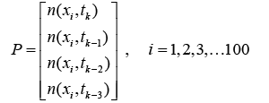
As shown in Figure 10, the input vector P is represented by the solid vertical bar at the left. The dimensions of P are displayed below the variable as 4 × 1, indicating that the input is a single vector of 4 elements:

(4.1)

As told before wound shape is supposed as a circle and R=10 mm. R is divided to 99 equal intervals. It means that there are 99 elements, and between x=0 and x=R there are 100 nodes. So:

(4.2)

(4.3)

These inputs go to the weight matrix W, which has 4 columns.

(4.4)

(4.5)

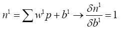
A constant 1 enters the neuron as an input and is multiplied by a scalar bias b. The net input to the transfer function f is n, which is the sum of the bias b and the product wp.

(4.6)

(4.7)

The neuron’s output a is a scalar in this case. If we had more than one neuron, the network output would be a vector. Here we have one output and it is the cell concentration amount in time step of k+1 (tk+1):

(4.8)

The main idea is by giving cell conservation at the t=k, t=k-1, t=k-2 and t=k-3 of each node to this neural network as a input vector, get the cell conservation amount at t=k+1.

For example to calculate the cell conservation in x=5 mm at t=104, n (5,104), as output of network we should give cell conservations in x=5 mm at t=100, t=101, t=102, t=103 as inputs of neural network, n (5,101), n (5,102), n (5,103), n (5,104) (Figure 13)

Figure 13: Cell conservation along R (number/ml).

Note that the number of inputs to a network is set by the external specifications of the problem; also, w and b are both adjustable scalar parameters of the neuron. That's how it works: usually the transfer function is picked by the designer and then the parameters w and b will be adjusted according to some learning rules so that the neuron input/ output relationship fulfills some special goal.

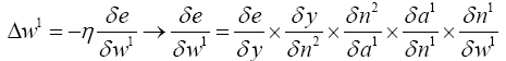
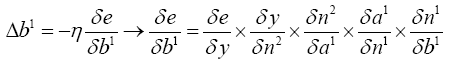
In this research, we use a training algorithm called backpropagation, which has told before is based on gradient descent.

Chain rule

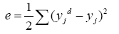
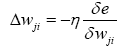
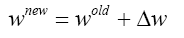
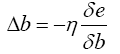
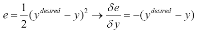
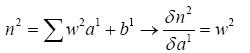
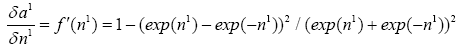
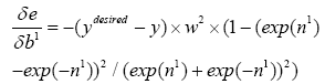
Before writing chain rule for each network we should be familiar with four important equations:

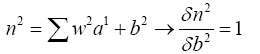
(4.9)

(4.10)

(4.11)

(4.12)

(4.13)

(4.14)

(4.15)

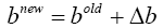
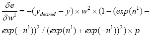
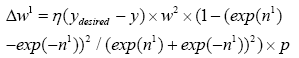
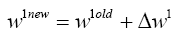
So, in each layer to find W^new and b^new, at first, we should calculate Δb and Δw.

Hidden layer:

a) Computing W^1new:

From (4.11) we know:

(4.16)

(4.17)

(4.18)

(4.19)

(4.20)

(4.21)

With substituting (4.17)-(4.21) in (4.16):

(4.22)

(4.23)

So we can now compute W^1new with replacing (4.23) in (4.13):

(4.24)

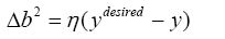
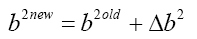
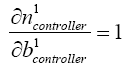
b) Computing b^{1 new}:

(4.25)

(4.26)

With replacing (4.17)-(4.20) and (4.26) in (4.25):

(4.27)

With replacing (4.27) in (4.14):

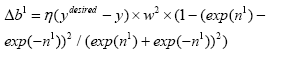(4.28)

So we can compute W^1new with replacing (4.28) in (4.15):

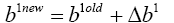(4.29)

Last layer:

a) Computing W^2new:

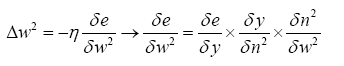(4.30)

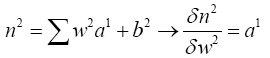(4.31)

With substituting (4.17) and (4.31) in (4.30):

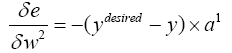(4.32)

With replacing (4.32) in (4.12):

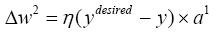(4.33)

So we can compute W1new with replacing (4.33) in (4.13):

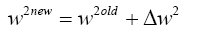(4.34)

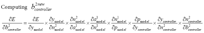
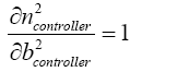
b) Computing b^2new:

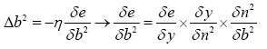(4.35)

(4.36)

With substituting (4.17) and (4.31) in (4.14):

(4.37)

With replacing (4.37) in (4.15):

(4.38)

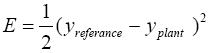
Figure 14 illustrates error of neural network's model for whole nodes at each time step converge to zero, so the output of the neural network has fairly no differences with plant's output. It means that this neural network model after training by back-propagation algorithm shows the same behavior as mathematical model and the output of neural networks is the same as plant's (mathematical model) output in each time step (Figure 15).

Figure 14: Plant's error along time.

Figure 15: Neural network's output R (number/ml).

Almost all tissue types have the ability to adapt to changes in the applied load, according to Wolff’s law [36]. The cells maintain the matrix and they are the key modulators of mechanically-induced tissue formation and remodeling, and in this way actively control tissue architecture and mechanics to adapt to changes in functional demands. The cells can reorganize and remodel the extracellular matrix by changing the production of matrix components, by secreting matrix enhancing or degrading products and their inhibitors, and by applying (traction) forces to the deposited fibers. At the moment, it is not exactly known how the cells sense and affect their environment, but several cellular mechano sensors and mechano transduction pathways have been proposed [37,38].

It is generally accepted that collagen synthesis, accumulation and organization are increased by mechanical stimuli, resulting in improved mechanical properties of the tissue. Cyclic strain increased the production of collagen in engineered smooth muscle tissue [39] and the rate of collagen synthesis was increased in mechanically stimulated in-vitro pulmonary arteries [40]. Collagen content also increased in long-term tissueengineered vascular structures [41] and in axially stretched in-vivo carotid arteries [42]. Pulmonary fibroblasts also showed an increased collagen expression when stimulated mechanically.

Increasing collagen content means increasing number of fibroblasts [33], so it can be said cell density (fibroblast density) can be increased by mechanical stimuli. This stimulation can be electrical stimulation or effect of magnetic fields on wounded area.

With these descriptions we use effect of mechanical stimuli at the wounded area to control the healing process. We suppose this stimulation is the force which is result of exposing skin in electrical or magnetic fields and effect of this force is cell production. We suppose the relationship between the exerted force to skin and cell production is a linear function as seen below:

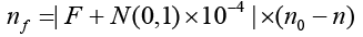(5.1)

Which N(0,1) is normal distribution with average zero and variance one.

nf is produced cell by exerted force to wound area, n0 is unwounded skin cell amount and n is cell amount which is produced by normal healing process and obtained from (3.1).

To control wound healing process (Figure 16) two networks are used, first one to simulate the plant and the second one acts as controller. These neural networks are two-layer networks; each layer has its own weight matrix W, its own bias vector b, the neural network used as plant's approximators has one input and one output and the other neural network used as controller has two inputs and one output. We will use superscripts to identify the layers. Specifically, we append the number of the layer as a superscript to the names for each of these variables. Thus, the weight matrix for the first layer is written as W1, and the weight matrix for the second layer is written as W².

Figure 16: Schematic of wound healing's controller.

Wound healings simulator

To model the plant, as told previously, consider a one hidden layer-network (Figures 16 and 17). This network has one input buffer (F) and single output (n). This network is trained online by getting force (F) data information executed from neural network controller, and approximates amount of cell (n) as networks output. Error will calculate by comparing neural network's output with plant's output as desired output. Desired output can be obtained in two ways:

Figure 17: Simulator of neural network's plant.

1. Using data information which is obtained by experience in real world.2. Using appropriate mathematical model.

For our purpose we choose the second one, so use mathematical model which introduced before, but this technique is established for real data instead of mathematical model. Nodes' weights and biases are updated by using error back propagation method and chain rule is written as same fashion as told before in section 4.

So input, output, bias and weight matrixes are defined (Figure 17).

(5.2)

(5.3)

(5.4)

(5.5)

(5.6)

(5.7)

Chain rules to back-propagate the error is written in the same fashion seen in section 4.

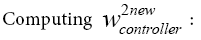
We choose model reference control (MRC) architecture to design neural network controller. This MRC controller is designed in the same fashion as plant approximator's network. The controller's network has two inputs, first one is error in k^th time step (E_k) which is calculated from difference between output of controlled plant, Cell (n), and amount of cell exists in unwounded (normal) skin (model reference), and the other one is derivative of Ek with respect to time (ΔE_k) (Figure 18).

Figure 18: Controller's neural network.

As told before the output of controller is force (F) established by magnetic or electrical field. Hence skin is exposed to this force the body autonomously starts producing cells (n_f) which results healing the scar tissue. So input, output, bias and weight matrixes are defined as seen below:

(5.8)

(5.9)

(5.10)

(5.11)

(5.12)

(5.13)

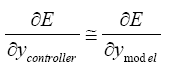
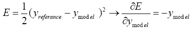
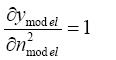
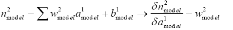
Chain rules for neural networks controller is written like chain rules for plant, but note that in back-propagating error of the controller and updating the hidden layer's weights matrix the output of controller (y_controller) in each time step is input of plant and as told before error of controller (E) is calculated from differences between output of plant and model

Reference so cannot be calculated directly. In the other hand it is known that the neural network used as plant approximators after training in each time step shows the same behavior as plant, it means that the output of plant and neural network used to simulated this plant are equal, so:

(5.14)

(5.15)

So:

(5.16)

So:

(5.17)

So, we can use instead of and chain rule for controller is written using data information of the neural network used as plant approximators as seen below.

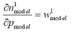
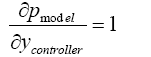
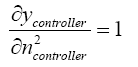
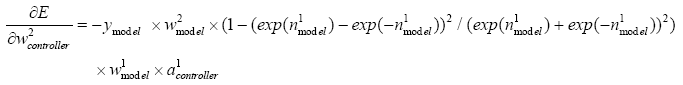
Last layer:

(5.18)

(5.19)

(5.20)

(5.21)

(5.22)

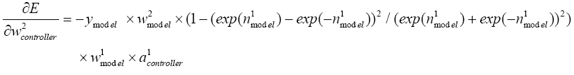
(5.23)

(5.24)

(5.25)

(5.26)

With replacing (5.19)-(5.26) in (5.18):

(5.27)

With replacing (5.27) in (4.12):

(5.28)

With replacing (5.28) in (5.13):

(5.29)

(5.30)

(5.31)

With replacing (5.19)-(5.25) and (5-31) in (5.30):

(5.32)

With replacing (5.31) in (4.14): (5.33)

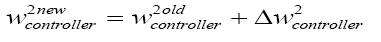
With replacing (5.33) in (4.15):

(5.34)

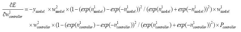
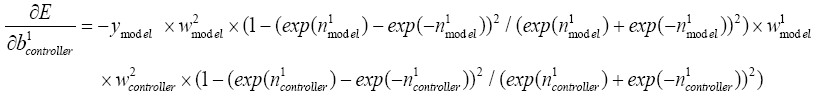
Hidden layer

(5.35)

(5.36)

(5.37)

(5.38)

With replacing (5.19)-(5.24) and (5.36)-(5.38) in (5.35):

(5.39)

With replacing (5.39) in (4.12):

(5.40)

with replacing (5.40) in (4.13):

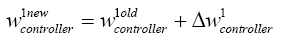(5.41)

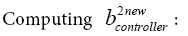
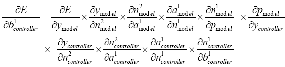(5.42)

(5.43)

With replacing (5.19)-(5.25), (5.36), (5.37) and (5.43) in (5.42):

(5.44)

With replacing (5.44) in (4.14): (5.45)

With replacing (5.45) in (4.15):

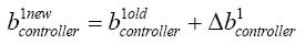(5.46)

We assume wound's shape as a circle (r=10 mm) with no cell at the center of it; if we start going further from the center to edges of the wound, increasing in cell amount will be seen. As told before controller's inputs are E_k and ΔE_k which at k=1 are given arbitrary. We assume these values 0.5 and 0.0 for E_k and ΔE_k respectively, and Controller's output is force (F) which is input of plant. Controller's neural network is trained after 13 steps (days), it means that after 13 days difference between output of controlled plant and model reference converge to zero also (Figures 19 and 20) error of plant's neural network in each time step (day) converge to zero it means that in each day plant's neural network show the behavior as plant (mathematical model). In this moment which controller is trained we can eliminate the model's neural network and test controller's network. Controller's inputs are E_k and ΔE_k with initial values of 1 and 0 w respectively (Figure 21). The output of controller is force (F) which also is plant's input (Figure 22). In each day (time step), executed force by controller is exerted to scar tissue and results in cell production in stimulated tissue (Figure 23). These produced cells resulted of exerted force to scar tissue are added to cells produced naturally in wound healing process, and make total cell content being in scar tissue which is plant's output. In Figure 24 it obviously can be seen by exerting appropriate force to scar tissue, body is forced to produce more cells in stimulated area, so number of cells in that area is increased. It means that by stimulating scar tissue, number of cells is fairly reached to model reference's cell number (normal skin, and results in reducing the scar tissue. It means that difference between total cell number and normal skin's cell, reduced and converges to zero (Figure 25). Healing process with controller is completely done within 37 days but in normal wound healing process cell number will be reached to normal skin's cell number after 1600 days (Figures 26-28).

Figure 19: Error of controlled plant and model reference (E).

Figure 20: Error of model's neural network along time (day).

Figure 21: Inputs of controller's neural network along time.

Figure 22: Exerted force to scar tissue: F (N).

Figure 23: Produced cells by exerted force to scar tissue: nf (number/ml).

Figure 24: Plant's output: total cell n (number/ml).

Figure 25: Error of controlled plant and model reference (E).

Figure 26: Dividing R to 3 equal intervals.

Figure 27: Dividing R to 9 elements.

Figure 28: Simulator of neural network's plant.

Control of wound healing by neural networks is a new idea discussed here as Bio-Control science. In this research we design a model free controller by neural networks (NNC) for wound healing procedure. In the procedure of control, after training of the NN controller, the neural networks of model will be eliminated. At any simulation by introducing a suitable reference model and by only measuring the cell content of skin as output we see that the healing process will be under control. Note that in control process we do not need to mathematical model equation anymore.

References

- Jennings RW, Hunt TK (1992) Overview of postnatal wound healing. In Fetal wound healing: Elsevier 25-52.
- Clark RAF (1996) Wound repair overview and general considerations. In the molecular and cellular biology of wound repair. Plenum Press, NY, USA.pp.3-50.
- Whitby DJ, Ferguson MWJ (1991) The extracellular matrix of lip wounds in fetal, neonatal and adult mice. Development 112: 651-668.
- Ehrlich PH, Krummel TM (1996) Regulation of wound healing from connective tissue perspective. Wound Repair Regen 4: 203-210.
- Gabbiani G, Majno G (1972) Dupuytren’s contracture: Fibroblast contraction? An ultrastructural study. Amer J Pathol 66: 131-146.
- Shuster S (1979) The cause of striaedistensae. Acta Dermato-Venereologica 59: 161-169.
- Stadelmann WK, Digenis AG, Tobin GR (1998) Physiology and healing dynamics of chronic cutaneous wounds. Am J Surg 176: 26S-38S.
- Diegelmann RF, Evans MC (2004) Wound healing: An overview of acute, fibrotic and delayed healing. Front Biosci 9: 283-289
- Martin P (1997) Wound healing-aiming for perfect skin regeneration. Science276:75-81.
- Arquilla ER, Weringer EJ, Nakajo M (1976) Wound healing: A model for the study of diabetic angiopathy. Diabetes25: 811-819.
- Kiecolt-Glaser JK, Marucha PT, Malarkey WB, Mercado AM (1995) Slowing of wound healing by psychological stress. Lancet 346: 1194-1196
- Pilcher BK, Wang M, Qin XJ, Parks WC, Senior RM, et al. (1999) Role of matrix metalloproteinases and their inhibition in cutaneous wound healing and allergic contact hypersensitivity. Ann NY Acad Sci 878: 12-24.
- Marucha PT, Kiecolt-Glaser JK, Favagehi M (1998) Mucosal wound healing is impaired by psychological stress. Psychosomatic Medi 60: 362-365.
- Forrest L (1983) Current concepts in soft connective tissue wound healing. Br J Surg 70: 133-140.
- Clark RAF (1996) The molecular and cellular biology of wound repair. NewYork: Plenum press, USA.
- Hay ED (1991) Cell biology of extacellular matrix, (2nd edn) New York: Plenum Press, USA.
- Hsieh P, Chen LB (1983) Behavior of cells seeded on isolated fibronectin matrices. J Cell Biol96: 1208-1217.
- Guido S, Tranquillo RT (1993) A methodology for the systematic and quantitative study of cell contact guidance in oriented collagen gels. J Cell Sci 105: 317-331.
- Clark P, Connolly P, Curtis ASG, Wilkinson CCW (1990) Topographical control of cell behavior. II. Multiple grooved substrata. Development 108: 635-644.
- Wojciak-Stothard B, Denyer M, Mishra M, Brown RA (1997) Adhesion orientation, and movement of cells cultured on ultrathin fibronectin fibers. In Vitro Cell Dev Biol 33: 110-117.
- Xu J, Clark RAF (1996) Extracellular matrix alters PDGF regulation of fibroblast integrins. J Cell Biol 132: 239-249.
- Clark RAF, Nielsen LD, Welch MP, McPherson JM (1995) Collagen matrices attenuate the collagen-synthetic response of cultured fibroblasts to TGF-b. J Cell Sci 108: 1251-1261.
- Ehrlich PH, Krummel TM (1996) Regulation of wound healing from a connective tissue perspective. Wound Repair Regen 4: 203-210
- Hsieh P, Chen LB(1983) Behavior of cells seeded on isolated fibronectin matrices. J Cell Biol 96: 1208-1217.
- Alberts B, Johnson A, Lewis J, Raff M, Roberts K, et al. (2002) Cell junctions, cell adhesion, and the extracellular matrix. In Molecular biology of the cell,(4th edn) New York: Garland Publishing, USA. pp.978-986
- Birk DE, Trelstad RL (1986) Extracellular compartments in tendon morphogenesis: Collagen, fibril, bundle, and macroaggregate formation. J Cell Biol 103: 231-240
- Bucalo B, Eaglstein WH, Falanga V (1993) Inhibition of cell proliferation by chronic wound fluid. Wound Repair Regen 1: 181-186.
- Mann BK, Schmedlen RH, West JL (2001) Tethered-TGF-beta increases extracellular matrix production of vascular smooth muscle cells. Biomaterials 22: 439-444.
- Streuli C (1999) Extracellular matrix remodelling and cellular differentiation. CurrOpi Cell Biol 11: 634-640.
- Hayashi K (1996) Biomechanical studies of the remodeling of knee joint tendons and ligaments. J Biomech 29: 707-716.
- Murray JD (2003) Mathematical biology II, (3rd edn). Springer Nature, NY, USA.
- Doillon CJ, Dunn MG, Bert RA, Silver FH (1985) Collagen deposition during wound repair. Scanning Electron Microsc 2: 897-903.
- Wolff J (1986)Â The law of bone remodeling (Das Gesetz der Transformation der Knochen). Berlin: Springer (Hirchwild), Germany.
- Tracqui P (1995) From passive diffusion to active cellular migration in mathematical models of tumour invasion. Acta Biotheoretica 43: 443-464.
- Chiquet M (1999) Regulation of extracellular matrix gee expressions by mechanical stress. Matrix Biol 18: 417-426.
- Kolpakov V, Rekhter MD, Gordon D, Wang WH, Kulik TJ (1995) Effect of mechanical forces on growth and matrix protein synthesis in the in-vitro pulmonary artery. Analysis of the role of individual cell types. Circulation Res 77: 823-831.
- Moses MA (2001) Dynamics of extracellular matrix production and turnover in tissue engineered cardiovascular structures. J Cell Biochem 81: 220-228.
- Jackson ZS, Gotlieb AI, Langille BL (2002) Wall tissue remodeling regulates longitudinal tension in arteries. Circu Res 90: 918-925.
- Breen EC (2000) Mechanical strain increases type I collagen expression in pulmonary fibroblasts invitro. J App Physiol 88: 203-209.
- Cukjati M, Robnik-Sikonja S, Rebersek D, Miklavcic I, Kononenko (2001)Prognostic factors in the prediction of chronic wound healing by electrical stimulation. J MedBiol Engineer Comput 39: 542-550.
- Canseven AG, Tohumoglu G, Abdükadir C, Nesrin S (2007)Explicit formulation of magnetic fields effects on skin collagen synthesis via neural networks.Int J Nat Engineer Sci 1: 119-125.
Citation: Azizi A (2017) Designing of Artificial Intelligence Model-Free Controller Based on Output Error to Control Wound Healing Process. Biosens J 6: 147. DOI: 10.4172/2090-4967.1000147
Copyright: ©2017 Azizi A. This is an open-access article distributed under the terms of the Creative Commons Attribution License, which permits unrestricted use, distribution, and reproduction in any medium, provided the original author and source are credited.
Select your language of interest to view the total content in your interested language
Share This Article
Recommended Journals
Open Access Journals
Article Tools
Article Usage
- Total views: 26622
- [From(publication date): 0-2017 - Dec 12, 2025]
- Breakdown by view type
- HTML page views: 25308
- PDF downloads: 1314