Journal of Earth Science & Climatic Change
Open Access

The attenuation of solar radiation through a real atmosphere versus that through a clean, dry atmosphere gives an indication of the atmospheric turbidity. I_T is a very suitable approximation to model the atmospheric absorption and scattering of the extraterrestrial radiation relative to dry and clean atmosphere [1]. Its study is important for monitoring atmospheric pollution trough the presence of dust aerosols in the meteorology and climatology. Atmospheric turbidity associated with aerosols from dust loads, water vapor and anthropogenic source is also an important parameter for assessing pollution trends [2].

As other published literatures, atmospheric aerosol has increased enormously over the last two decades. I_T can either have nonanthropogenic or anthropogenic sources and are either emitted as primary particles (i.e. They are directly emitted to the atmosphere) or formed by secondary processes (i.e. By transformation of emitted precursor gases). I_T has been rising from low concentration over the preserved forest of Amazonian because of land-use change from natural begins to biomass burning [3] may bring T_L to the pollution level. According to Engelbrecht and Derbyshire [4] the pollution level of dust aerosols through the determination of T_L being closer to 8.

The global source regions of dust have covered the Northern Hemisphere, including North Africa, the Middle East, the Northwest Indian subcontinent, central Asia, and Northwest China [4]. Ethiopia is not immune from the large influx of dust because of its proximity, particularly in the Sahel and Arabia Peninsula. Influx dust from these regions, particulate matter from nearby industries, and smokes from deforestations for agriculture and fuel wood combined with maritime (Red Sea and Indian Ocean) moisture may contribute the rise of a turbidity factor in the area. The study area for this purpose is an Illusanbitu District located in tropical highland of South-East Ethiopia at about 7° latitude, 40° longitudes and 2500 m altitude. The determination of Linke’s turbidity factor T_L was carried out from three method data.

• The meteorological data on Global Solar Radiation (GSR) were obtained from a non-government organization called Africa Rising [5] settled there.

• The model GSR data were extracted through integrating of mathematical equations from four atmospheric parameters by MATLAB tool.

• The satellite GSR data at the location was freely logged down from a website called Atmospheric Science Data Center controlled by the National Aeronautics and Space Administration NASA.

Mathematical formulations for global solar radiation modeling

The mathematical formulations were largely reviewed from the book written by Iqbal [6], and some published journals listed in the reference. The modeling in determining GSR entirely depends upon integrating the four major classifications of atmospheric parameters discussed below:

a. Geographical Parameters: The altitude and latitude in combining solar geometry climatic and optical parameters are essential in determining the amount of solar insolation reaching the earth’s surface.

b. Solar Geometric Parameters: Under this category, the amount of solar irradiance reaching the study area are influenced by solar geometry parameters such the solar zenith angle θ_z , declination angle δ solar altitude angle η and solar hour angles ω . The solar geometry called declination angle δ is computed as:

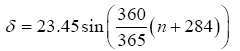(1)

The orientation of a horizontally placed solar receiver towards the incident radiation related to the declination angle δ , solar zenith θ_z , latitude ϕ, solar altitude angle η and solar hour angle ω in degree related as:

(2)

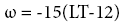(3)

Where L_T is the local time from the midnight. On the other hand, I_T is well known that atmospheric turbidities linked with the presence of aerosols, water vapor, and ozone are the most important extinction components affecting the direct and diffuse components of solar radiation under clear skies [7]. As a matter of fact, the effect of moist or water vapor is taken by considering the w in centimeter in terms, relative humidity H_r, ambient temperature T and partial pressure in Kelvin are expressed in Equations 4 and 5.

a. Climatic parameters: These classifications involve the measurement of ambient temperature, relative humidity, horizontal climate visibility and partial air pressure. The ambient temperature and relative humidity are also served for computing perceptible water vapor w using Equations 4 and 5. As a matter of fact, the effect of moist or water vapor is taken by considering the w in centimeter in terms, relative humidity, H_r ambient temperature T and partial pressure in Kelvin are expressed in these equations.

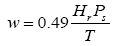(4)

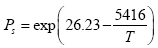(5)

The horizontal visibility V is also a significant climate factor in computing optical air transmittance in Equation (6). The horizontal Vis of the area lies within the range of 17 km up to 22 km during winter when there are low rainfall and cloud coverage.

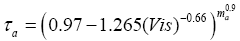
b. Atmospheric optical parameters: I_T is the most complex atmospheric phenomena in determining the energy budget at a given location. The amount of solar energy reaching the surface is affected by optical properties of water vapor, air, ozone layer and aerosol masses. Their effects on solar irradiance are sensed by computing their optical transmittance, reflectance, absorbance, Rayleigh centeredness and turbidity coefficients that attenuate the solar irradiance reaching the surface. The ground albedo is also taken into consideration for modeling purposes. The computed value of relative optical masses of aerosol τ_a , air mass m_a, water vapor m_w and ozone m_o at a given location are given under Equations (6), (7) (10) and (11) respectively. Their values are almost in closer ranges as stated by Iqbal [6]. However, an optical mass of aerosols m_o is the most uncertain parameters in calculating solar radiation on the ground [6]. They are highly variable in size, distribution, composition, and optical properties. For lack of required information, the value of computing optical air mass m_a can be used as a substitute for optical mass of aerosol m_o in Equation (7). Therefore, the optical transmittance τ_a written in Eq. (6) as the presence of aerosols is calculated as

(6)

Where m_a is in the Equation (6) is the relative optical dry air mass for local conditions computed through Equations 7, 8, and 9.

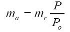(7)

Where P and P_o are the local pressure and sea level pressures in millibars respectively. The local atmospheric pressure above sea level at altitude z is evaluated as:

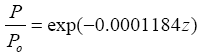(8)

The altitude of the study location z is around 2480 m. The relative optical air mass m_r in Equation (7) may be approximated by relating to zenith angle :

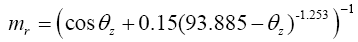(9)

On the other hand, the corresponding expressions for relative optical water vapor mass m_w and relative optical ozone mass m_o are expressed in the following two expressions by Iqbal.

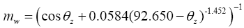(10)

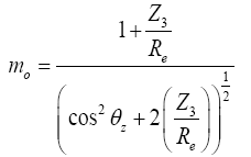(11)

Where Z₃ measures the concentrated ozone at around 22 km and R_e is the radius of the earth approximated as 6370 km. Overall spectrally integrated transmittance computation for each atmospheric constituent is necessary steps for solar radiation parameterization in modeling [7]. The total transmittance τ as a function of the ozone layer thickness in cm, perceptible water vapor w in cm, turbidity coefficient β and α , and the relative mass is evaluated by Iqbal [6]:

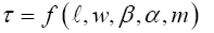(12)

The transmittance quantities and for some major atmospheric constitutes such as water vapors, ozone layers and aerosols are expressed as respectively in Equations (13), (16) and (28).

(13)

Where α_w is the attenuation coefficient of water vapor given as:

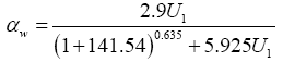(14)

Where U₁ is the pressure-corrected relative optical path length written in terms of m_r and w as:

(15)

The transmittance due to the ozone layer is given as:

(16)

Where α_o is the attenuation coefficient due to direct irradiance transmission through the ozone layer. Its expression is written as:

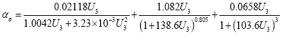(17)

The U₃ is the ozone relative optical path given by:

(18)

For broad spectral range, the integrated transmittance for Rayleigh scattering over the wavelength interval is defined as (Iqbal, 2012)

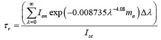(19)

I_on is the direct irradiance on horizontal surface normal to the sun's rays (also called direct normal radiation) and I_sc is the solar constant whose value is 1367 W/m². A regression-type correlation that fits Equation (19) is given as:

(20)

During parameterization of the solar radiation, the direct normal irradiance I_on on a horizontal surface at a zenith angle at mean sunearth distance by including the correction factor called eccentricity can be given by Iqbal [6]:

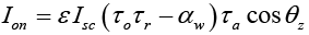(21)

Where the eccentricity correction factor related to the number n of days in the year is given by:

(22)

Therefore, the total global irradiance I_T on a horizontal surface from direct irradiance and diffused irradiance I_d from surrounding environment can be written as follows:

(23)

The I_d can be further written as:

The broadband diffuse irradiance I_dr under a cloudless sky as the effect of Rayleigh scattering is given as

(25)

On the other hand, the diffuse irradiance scattering because of aerosol-scattered diffuse radiation I_da reaching the ground after the first pass through the atmosphere is given as

(26)

Where F_c is symbolized for forward scattering, is symbolized for the single scattering albedo by Iqbal, which is the ratio of energy scattered by aerosol to the total attenuation under primarily incident by the direct radiation. In this paper a value of [6] was taken for the computation. The determination of is experimentally a troublesome, according to Iqbal [6]. However, a few amount of aerosol particles in rural environment usually scattered than those found in the urban-industrial area [6,8]. During solar irradiance modeling = 0.6, by Iqbal [6] is used for urban-industrial region where as = 0.9 [6,8] is used for agricultural region. Since the study location is widely known as the rural and agricultural center, so = 0.9 was applied in the solar radiation modeling. The horizontal visibility (Vis) for greater than 5 km, Ångström turbidity factorβ , and wavelength exponent α are related as:

(27)

The wavelength exponent α = 1.3 in Equations (27) and (28) was used in the computation according to Iqbal [6]. The aerosol transmittance τ_a' computed using air-mass m'_a, Ångström turbidity factor β , and wavelength exponent α is:

(28)

Where m'_a is the relative aerosol mass at the local station calculated as:

(29)

The downward irradiance I_dm because of multiple reflections between the ground and the atmosphere is computed as:

(30)

Where ρ_g is the ground albedo and ρ_g ′ is cloudless sky albedo. The value of ground albedo for variation of multiply reflected irradiance lies between 0.2 and 0.7 according to Iqbal [6]. On another reference, the ground albedo varied between 0.1 and 0.25 for agricultural and grassland is written in Encyclopedia of Soil Science. In this paper 0.25 ρ_g = was used for computing the downward irradiance I_dm due to multiple reflections between the ground and the atmosphere. The cloudless sky albedo a ρ ′ is computed as Figures 1 and 2

Figure 1: The estimation of precipitable water vapor w using Equations 3 and 4.

Figure 2: Ground measurement of GSR.

(31)

Determination of linked turbidity factor T_L

The influence of T_L on GSR at site were evaluated by Inman and Becker [9,10]:

(32)

Where is the Rayleigh optical thickness. I_T was employed in evaluating T_L were referenced by Inman [9]:

Its equation is represented as:

(33)

(34)

The is computed according the condition set by Wang, Chen, Niu, Salazar [11]. According to them is to be greater than 10⁰, I_on is to be greater than 200 W/m² and the is to be less than 20.

(35)

The T_L illustrated on Figures 3-7 is from modeled GSR oscillated between 4.2 and 8.2 with its mean value about 6.2. The T_L from GSR of ground measurement is oscillated between 3.6 and 8.4 with mean value 6.16.

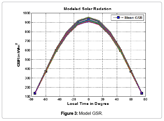
Figure 3: Model GSR.

Figure 4: Comparison of mean, modal, median, and 15th day (January 2016) of ground measurement with model GSR.

Figure 5: Mean daily GSR from modelling, ground measurement and satellite reading.

Figure 6: The T_L from GSR modelling and ground measurement.

Figure 7: Daily determination of L T ’s with their means (model, measurement and satellite).

The statistical tools for evaluating hydrological model assessment widely discussed by Krause, Boyle, Bäse [12], where applicable for evaluating the model efficiency in determining T_L . These are: Root Means Squared Error RMSE, Nash-Sutcliffe efficiency E and its relative efficiency criteria E_r, index agreement d and its relative efficiency criteria d_r and coefficient of determination R².

An efficiency of 0 indicates that the model predictions are as accurate as the mean of the observed data, whereas an efficiency less than zero ( −∞ < E < 0) occurs when the observed mean is a better predictor than the model. Essentially, the closer the model efficiency is to 1; the model is becoming more accurate. On the other statistical explanation on modeling, the coefficient of determination R² ranging between 0.33 and 0.66 would have moderate explanatory power [13].

As I_T is seen in Figure 7 the daily T_L from model GSR is smoothly varied between 6.02 and 6.34 with mean 6.22. However, the daily T_L from ground GSR is considerably varied between 3.62 and 8.36 with the daily mean ranging between 5.77 and 6.71. The daily T_L from satellite GSR is also dramatically varied between 3.51 and 8.02 with daily mean lies between 5.12 and 6.01.

The model GSR for the study is computed from integrated atmospheric parameters such as optical thickness, optical air mass, and ozone layer, the amount of aerosol effect, perceptible water vapor, climate data, solar geometry and geographical positions. This rise of Like’s turbidity factor is an outcome of the suspension of particulate matters, smokes and water droplet in the atmosphere. The area’s proximity to Sahel and Arabia Peninsula, large influx of dusts can stream in to I_T . Maritime moisture from Red Sea and Indian Ocean combined with the dusts, particulate matters from local industries, smokes from traditional energy consumption patterns may bring the turbidity factors to the pollution level assisted through local and global wind system transport. These would have consistent pressure on the sustainability of water, air, and soil quality in the area. The T_L from the model, ground and satellite GSR is approximately in a close agreement varied between 4 and 8 with the daily average 6 point. This rise of T_L is approximately laid in the range between 20% to 37.5% as compared to T_L of tropical warm air (continental) in 1947 as discussed by Becker [10]. The result is almost in closer agreement with the analysis made in other continent (Asia) by Wang, Chen, Niu and Salazar [11], Computing the Like’s atmospheric turbidity is an important procedure for early warning on monitoring air, water, soil quality for stability of healthy ecosystem.

The author appreciates and acknowledges heartily the teams in Africa Rising for providing meteorology data to academic researchers.

References

- Marif Y, Bechki D, Zerrouki M, Belhadj MM, Bouguettaia H (2017) Estimation of atmospheric turbidity over Adrar city in Algeria. Journal of King Saud 17: 1333-1317.
- Abdelrahman MA, Said SAM, Shuaib AN (1988) Comparison between atmospheric turbidity coefficients of desert and temperate climates. Solar Energy 40: 219-225.
- Fuzzi S, Baltensperger U, Carslaw K, Decesari S, Denier Van DGH (2015) Particulate matter, air quality and climate: Lessons learned and future needs. Atmospheric chemistry and physics 15: 8217-8299.
- Engelbrecht JP, Derbyshire E (2010) Airborne mineral dust. Elements 6: 241-246.
- Kemal SA (2017) Africa rising Ethiopia highlands final technical report January 2012 September 2016.
- Gueymard CA (2005) Importance of atmospheric turbidity and associated uncertainties in solar radiation and luminous efficacy modelling. Energy 30: 1603-1621.
- Fraser RS, Kaufman YJ (1985) The relative importance of aerosol scattering and absorption in remote sensing. IEEE Transactions on Geoscience and Remote Sensing 5: 625-633.
- Inman RH, Edson JG, Coimbra CF (2015) Impact of local broadband turbidity estimation on forecasting of clear sky direct normal irradiance. Solar Energy 117: 125-138.
- Becker S (2001) Calculation of direct solar and diffuse radiation in Israel. International Journal of Climatology 21: 1561-1576.
- Wang L, Chen Y, Niu Y, Salazar GA (2017) Analysis of atmospheric turbidity in clear skies at Wuhan, Central China. Journal of Earth Science 28: 729-738.
- Krause P, Boyle DP, Bäse F (2005) Comparison of different efficiency criteria for hydrological model assessment. Advances in geosciences 5: 89-97.
- Huang CC, Wang YM, Wu TW, Wang PA (2013) An empirical analysis of the antecedents and performance consequences of using the moodle platform. International Journal of Information and Education Technology 3: 217.
Citation: Ambaye C (2018) Determination of Linke’s Turbidity Factors from Model and Measure Solar Radiations in the Tropics Over Highland of South-East Ethiopia. J Earth Sci Clim Change 9: 479. DOI: 10.4172/2157-7617.1000479
Copyright: © 2018 Ambaye C. This is an open-access article distributed under the terms of the Creative Commons Attribution License, which permits unrestricted use, distribution, and reproduction in any medium, provided the original author and source are credited.
Select your language of interest to view the total content in your interested language
Share This Article
Recommended Journals
Open Access Journals
Article Tools
Article Usage
- Total views: 4690
- [From(publication date): 0-2018 - Aug 07, 2025]
- Breakdown by view type
- HTML page views: 3776
- PDF downloads: 914