Downscaled Projected Climate Scenario of Talomo-Lipadas Watershed, Davao City, Philippines
Received: 04-Mar-2015 / Accepted Date: 23-Mar-2015 / Published Date: 30-Mar-2015 DOI: 10.4172/2157-7617.1000268
Abstract
General Circulation Models (GCMs) are widely used tools to assess potential global climate impacts. However, GCMs’ outputs are difficult to use in regional impact studies because of their coarse spatial resolution; it is much more difficult at local level climate impact assessments. Hence, downscaling techniques are applied to bridge the spatial and temporal resolution gaps between what climate modellers are currently able to provide and what impact assessors require. The study aims to downscale station -scale climate scenarios in Talomo-Lipadas Watersheds, Davao City, Philippines for the years 2020, 2050, and 2080 under two scenarios (A1B and A2). It quantifies the increase/decrease of minimum temperature, maximum temperature, and precipitation. For the two watersheds under study, temperature minimum (Tmin) results show a likely slight increase from 0.159°C to 0.239°C; Tmin also shows an increasing trend under two scenarios (A1B and A2). For temperature maximum (Tmax), the two watersheds will experience prolonged periods of hotter temperature. For precipitation, simulated result shows heavy rainfall of 42.87% above observed data under A1B scenario. At the onset of the year, the two watersheds will experience wetter conditions in two scenarios. A1B scenario is projected to be “wetter” compared to A2 scenario. The highest rainfall of 335 mm is observed in June of 2050 (2041-2070) slice time period.
Keywords: SDSM; Statistical downscaling; Davao watersheds; Projected climate; Talomo-Lipadas; Davao climate
8888Introduction
Background of the study
Downscaling station-scale climate scenario is one of the most challenging yet useful tools in addressing climate change impacts. Powerful and down to earth climate change scenarios are at the heart for the success of Vulnerability and Adaptation assessments. This is largely because of the usefulness of the scenarios themselves in shaping and guiding Vulnerability and Adaptation Assessments [1]. A downscaled local climate scenario projection is a necessity for long-term planning. It enables the various sectors at the local level to define more clearly and accurately climate vulnerability and resiliency, appropriate adaptation strategies, and disaster risk reduction actions or programs.
General circulation models: Presently, GCMs are fundamental tools to predict the evolution of climate in the future. However, currently, General Circulation Models (GCM) describe only large scale global motions to capture long term changes in the atmosphere; GCMs provide low resolution information on 300 km scale; and, it has limited use when impact assessment is focused to future climate projections at regional and local scales.
What is needed is a much finer resolution at station-scale; whatever adaptation strategies on the table would likely fit and address the potential impacts posed from a changing climate.
Statistical Down Scaling Model (SDSM): Statistical Down Scaling Model (SDSM) is powerful software that can define and model future climate changes at finer resolution in local or individual sites. Downscaling techniques are used to bridge the spatial and temporal resolution gaps between what climate modellers are currently able to provide and what impact assessors require [2]. Statistical downscaling methodologies have several practical advantages over dynamical downscaling approaches. It represents a more promising option in situations where low–cost, rapid assessments of localized climate change impacts are required. It enables the construction of climate change scenarios for individual sites at daily time–scales, using grid resolution GCM output.
Talomo-lipadas watersheds: Talomo-Lipadas Watersheds, the subject of this study, is located in Davao City, Philippines. Specifically, it is situated in latitude of 07°08'02" and 07°09'14", respectively and a longitude of 125°20'50" and 125°29'01", respectively. Talomo- Lipadas watershed has a total land area of 38,375 hectares. These two watersheds are part of eight (8) sub-watersheds of Davao Greater Watershed. It covers the districts of Baguio, Calinan, Toril, Talomo, and Tugbok [3]. Presently, these watersheds are in varying stages of deterioration. Various pressures have been attributed to changing land uses, rapidly expanding population, pollution and etc. Most of the agriculture-related transnational companies have inhabited the Davao Region because of conductive climatic conditions, edaphic factors, and vast tracks of land [3]. Water demands of these companies contributed to the degrading water supplies not to mention the diminishing water quality specifically trace amounts of pesticides in drinking water, fertilizers, among others. These watersheds have long been the priority for management and development [4] since it is the main source of groundwater extraction that supplies a significant percentage of the water needs of Davao City. The results of this study are important to local water managers, water-users, and policy makers. The results will help shape robust planned adaptation strategies to address the looming water crisis in Davao City. Moreover, the output is important to all climate-dependent sectors like; DCWD, agriculture, hydropower plants in which the result will prepare them to potential negative and positive impacts of climate change.
Research problem
The Second National Report on Climate Change projected a hotter climate in Mindanao in the future. Philippine Atmospheric, Geophysical, and Astronomical Services Administration (PAGASA) also predicted an increase of temperature and a decrease of precipitation under medium scenario for the next 30 years or by 2050 [5]. Projections of both studies used GCMs at national and regional scales. This study will try to fill the gap, that is, to downscale climate scenario at station level. Then, it will attempt to measure how much is the increase/decrease of temperature and of precipitation projections under two scenarios. This study would project a downscaled climate scenario in three time slice periods, that is, 2020, 2050 and 2080 of the watershed area.
Objectives
General objective: This study aims to develop a downscaled projected station-scale climate scenario of Talomo-Lipadas Watersheds, Davao City, Philippines.
Specific objectives:
The specific objectives of this study are:
1. Develop a downscaled projected climate station scale of Talomo- Lipadas Watershed using Statistical Downscaling Method;
2. Evaluate the increase/decrease of local temperature both minimum and maximum as well as the increase/decrease precipitation in three time slice periods: 2020, 2050, and 2080; and
3. Assess how much is the increase/decrease of temperature and precipitation under two scenarios.
Research questions
This study seeks to answer the research questions to meet the research objectives.
1. Based on the Statistical Downscaling Method (SDSM) version 4.2.7, what is the downscaled projected climate station-scale of Talomo-Lipadas Watershed?
2. What is the increase/decrease of local temperature both minimum and maximum as well as the increase/decrease precipitation in three time slice periods 2020, 2050, and 2080?; and
3. What is the difference of increase/decrease of temperature and precipitation under two scenarios (A1B and A2)?
Significance of the study
Global climate models are readily available worldwide; however, there is a need to downscale the results at individual sites or localities for impact studies. In the Philippine context, only limited information is available and few studies conducted in relation to downscaling and projecting climate scenarios at station scale. The result of this study is also very important for all planners especially in water-related sectors like agriculture, domestic water users etc., to assess projected impacts and plan adaptation strategies and actions.
Intergovernmental Panel for Climate Change (IPCC) Fourth Assessment Report key findings concluded with “high confidence” that recent regional changes in temperature have had discernible impacts on physical and biological systems” [6]. The report has also observed a notable lack of geographic balance in data and literature on observed changes, with marked scarcity in developing countries like the Philippines. The assessment also highlighted the limits of integrated assessment of vulnerability and the limited understanding on how development planners incorporate and integrate information about climate variability and change into their decisions. Thus, this study would like to address these gaps by using downscaling methods of future climate scenario specifically at Talomo-Lipadas Watershed, Davao City, Philippines. Output of the study will be useful input for conducting a more robust and meaningful vulnerability and adaptation assessments.
Scope and limitation of the study
Statistical Downscaling Model Software (SDSM) version 4.2.7 is used in downscaling local climate scenario at the study area. Sets of predictor variables from National Center for Environmental Prediction (NCEP) as well as the Coupled Global Climate Model 3 (CGCM3) are downloaded via http://loki.qc.ec.gc.ca/DAI/predictors-e.html. Predictands such as daily precipitation, minimum temperature, and maximum temperature weretaken at Bago Oshiro Agro meteorological Station, Bago Oshiro, Tugbok District, Davao City. Said parameters and missing data were checked, counterchecked and verified at the PAGASA Central office, Agham Road, Quezon City. Weather projections of likely local climate are taken into three slice periods: 2020, 2050, and 2080 under two Special Report Emission Scenarios (SRES) scenario namely, A1B and A2.The study started from January and ended in June 2013.
Review of Related Literature
Because any policy research outputs using CGMs is linked to decision-makers mainly from government and industry, it is very important that the climate scenarios be plausible and that key uncertainties be presented in the output for possible adaptation planning. However, many regional and local climate/weather users have long been dissatisfied with the output specifically on the inadequate spatial scale of climate scenarios produced from coarse resolution global climate model (GCM) [7-11]. This is due to the perceived mismatch of scale between coarse resolution GCMs (100s of km) and the scale of interest for regional impacts [12,13]. SDMS have emerged to bridge climate macro and micro scale projections relating regionalscale atmospheric predictor variables to local-scale surface weather.
Coupled Global Climate Model 3 (CGCM 3)
Coupled Global Climate Model (CGCM3) is the third version of the Canadian Centre for Climate Modeling and Analysis (CCCma). This is the improved version that makes use of the substantially updated atmospheric component AGCM3 (Atmospheric Canadian GCM, version 3) that includes a new module for treatment of the land surface processes new treatment of water vapour transport; and cumulus parameterization. On the other hand, Coupled Global Climate Model 3 (CGCM3) model has been developed by the Canadian Centre for Climate Change Modeling and Analysis (CCCma) and can run to cover from the period of 1960 up to 2100 years. Datasets for the future period follow two SRES GHG+A scenarios A2 and A1B. The Canadian Climate Change Scenarios Network provides datasets that can be used as predictors for statistical downscaling [14]. All National Center for Environmental Prediction (NCEP) and National Center for Atmospheric Research (NCAR) data have been averaged on a daily basis from 6 hourly data, before being linearly interpolated to match the CGCM3 data. Where variables are derived, they are computed on the native 2.5° lat. x 2.5° longitude regular Gaussian grid, and then interpolated. As for spatial and temporal coverage, the CGCM3 T47 historical simulation and future runs together cover the entire period from 1961 to 2100 (1961-2000 and 2001-2100, for current and future time windows, respectively). Datasets for the future period follow two SRES GHG+A scenarios A2 and A1B (both the 4th member CGCM3 model runs). This is one of the models used in the fourth assessment report of IPCC in generating future climatic scenarios (Figure 1).
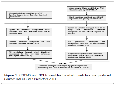
Figure 1: CGCM3 and NCEP variables by which predictors are produced Source: DAI CGCM3 Predictors 2003.
Statistical Down Scaling Model (SDSM)
Statistical down Scaling Model (SDSM) is a windows-based decision support tool for the rapid development of single-site, ensemble scenarios of daily weather variables under current and future regional climate forcing. This model has been widely used worldwide and in the Philippines in particular. SDMS have emerged as a means of relating regional-scale atmospheric predictor variables to local-scale surface weather. It is analogous to the ‘Model Output Statistics’ (MOS) and ‘perfect prog’ approaches used for short-range numerical weather prediction [15]. This approach will continue to play a significant role in the assessment of potential climate change impacts arising from future increases in greenhouse-gas concentrations [16]. One of the primary advantages of this statistical modelling technique is that SDSM is computationally inexpensive, and thus can be easily applied to output from different GCM experiments. SDSM can also be used to provide specific local information (e.g., points, catchments), which can be most needed in many climate changes impact studies. The applications of downscaling techniques vary widely with respect to regions, spatial and temporal scales, type of predictors and predictands, and climate statistics [17]. SDSM procedure starts with the assemblage of coincident predictor and predictand data sets. Predictands are individual daily weather series obtained from meteorological observations (Precipitation, Tmax, Tmin, hours of sunshine, wind speed, etc. These parameters do not limit to other environmental predictands (air quality parameters, sea levels, snow cover, etc. [18]. The next step of statistical downscaling is a two-step process, that is, i) development of statistical relationships between local climate variables (e.g., surface air temperature and precipitation) and large-scale predictors, and ii) application of such relationships to the output of GCM experiments to simulate local climate characteristics. Downscaling is justified when GCM (or RCM) simulations of the required surface variable(s) are un realistic at the temporal and spatial scales of interest—either because the impact scales are below the climate model’s resolution, or because of model deficiencies—yet are considered realistic at larger scales and/ or for other related variables. The choice of downscaling technique is governed largely by the availability of data for model calibration, and by the variables required for impact assessment. The same predictors should be available for target regions from both observed and GCM data (Figure 2) [2]. For the last few years, progress have been achieved on the extension of many downscaling models from monthly and seasonal to daily time scales, which allows the production of data more suitable for a broader set of impact assessment models (e.g., agriculture or hydrologic models) (Figure 3). Statistical downscaling models have been quite successful in achieving various statistics of local surface climatology [19]. Limited applications of statistical downscaling models to the generation of climate change scenarios has occurred showing that in complex physiographic settings local temperature and precipitation change scenarios generated using downscaling methods were significantly different from, and had a finer spatial scale structure than, those directly interpolated from the driving GCMs [19]. From a scientific perspective, models are valuable as tools to assist in interpreting data and in linking physical processes that are measured from the stand level to the watershed scale [20-23]. From an operational perspective, models are valued for their scenario analysis and predictive capability that enables resource managers in industry, government, and other sectors to predict what future watershed conditions might be under varying management practices. Models can also be used to account for complicating factors such as the effects of climate variability and climate change, or other disturbances in longterm planning.
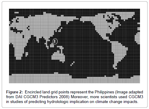
Figure 2: Encircled land grid points represent the Philippines (Image adapted from DAI CGCM3 Predictors 2008) Moreover, more scientists used CGCM3 in studies of predicting hydrolologic implication on climate change impacts.
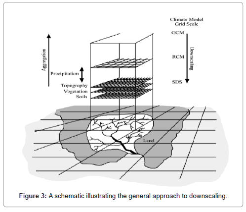
Figure 3: A schematic illustrating the general approach to downscaling.
Conceptual framework
Measham et al. [24] States: “the more the information is specific, the more powerful this became in terms of making a case for adaptation through planning.” Adaptation is local. The impacts of climate change are experienced locally, and therefore, geographic variability in climate impacts emphasises the need for ‘place-based’ approaches to climate vulnerability analysis and adaption [25-27]. This study anchored on above studies which summarize the need of climate information at finer resolution with spatial and temporal scales information for the precise nature of the conditions that needs to be adapted to. Figure 4 illustrates the conceptual framework of the study.
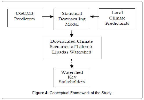
Figure 4: Conceptual Framework of the Study.
Study area and materials
Description of study site: The PAG-ASA weather station lies on 07°04’ 06” and 125°27’99”. This weather station has been in operation since May 1976 and situated within the Talomo Watershed within the Philippine Coconut Authority (PCA), Bago Oshiro, Davao City. Groundwater from Talomo-Lipadas Watersheds have been the primary source of drinking water for the entire city since the establishment of water district in 1973 [3]. It supplies 90% of the drinking water serviced by Davao City Water Districts [10]. And lastly, the area is a home of the famous endangered bird, Philippine Eagle (Pithecophaga jeferryi) (Figure 5).

Figure 5: Talomo-Lipadas Watershed, Davao City, Philippines.
Data collection: Climate data were taken from Philippine Atmospheric Geophysical and Astronomical Services Administration (PAGASA) Agrometeorological Station at Bago Oshiro, Tugbok District, and Davao City. Climate Data collected are: precipitation, temperature (maximum), temperature (minimum), and sunshine duration covering the period from 1976-2012 on daily time series. The data were cross-checked at PAGASA Central Office located at Agham Road, Quezon City. Other significant data, information, shape files for maps, and other relevant information were accessed through respective offices. Data gathering started from June 2012 and ended in February 2013.
Methodology
Statistical downscaling
The study follows the user manual of Statistical Downscaling procedure in generating the downscaled climate scenario at stationscale projection [18]. Statistical Downscaling Model (SDSM) using multiple linear regression was used in generating current and projected climate scenarios in three time slice periods specifically 2020 (2011-2040), 2050 (2041-2070) and 2080 (2071-2100). Calibration and validation determine the best fitted model and be able to use in projecting climate scenarios. The SDSM software reduces the task of statistically downscaling daily weather series into seven discrete steps. The procedure is shown below as adapted to SDSM Manual.
Quality control and data transformation: The weather station started its operation in collecting climate data in May 1976; hence, it had 37-years data collection until present. However, data sets were not totally complete hence, quality control were undertaken. Said data were validated at the PAG-ASA central office, Agham road, Quezon City. This procedure is necessary to ensure quality control.
Screening of predictor variables: Identifying empirical relationships between gridded predictors and single site predictands (such as station precipitation) is central to all statistical downscaling methods. Screen Variables operation was used to select the appropriate predictor variables. This is critical in developing statistical downscaling model wherein the selection of predictors determine the character of downscaled climate scenario. Predictors from global climate model were carefully selected vis a vis with predictands of local climate data in order to be processed. Although users can select predictors that are physically sensible prior to the conduct of Screen Variables, correlation analysis was used in selecting the predictors that are significant and highly correlated to the predictands. Selected variables were then used in model calibration.
Model calibration: Calibration of the model was done to generate the monthly structured models. Twelve various multiple linear regression models representing each month with different parameters was used in the model structure. Different models were created for each month as temporal variability was considered during the model building. Adjusting the value of the variance inflation was also made until the simulated data capture the monthly trends of the observed data. Maximum and minimum temperatures were modelled based on unconditional processes in which a direct link between the predictors and predictands were assumed. On the other hand, precipitation was modelled based on conditional process in which local precipitation amounts are correlated with the occurrence of wet days, which in turn is correlated with large scale atmospheric variables. Due to unavailability of climate data, the model calibration covers only for 20 years (1976- 1995) while the validation covers 12 years (1989-2000). Also, cross validation was applied [28,29]. The significant predictors selected during model calibration for each month was used in model validation. Multiple ensembles of downscaled weather data were generated based on the range of data used in model validation.
Weather generation (using observed predictors): Weather generator produced multiple ensembles of downscaled simulated/ generated daily data. Each ensemble has same plausible statistical characteristics but differ on day to day values. However, 30 ensembles were created to match the number of years for the observed data and time slices for future scenarios. The average value of the 30 ensembles was used in model evaluation. Independent downscaled data were generated from each dependent variables/predictands (minimum temperature, maximum temperature and rainfall) under different climate scenarios (NCEP reanalysis and CGCM3). Evaluation of the model and residual analysis was performed to analyze the performance of the model.
Statistical analyses: For this study, the adequacy of the model (R2) and deviation of the simulated data to the observed data using Root Mean Square Error (RMSE), Mean Absolute Error (MAE) and Nash- Sutcliffe Efficiency (E) were used in model evaluation.
Graphing model output: Observed and simulated data were compared through graphical presentation. Overestimation and underestimation can easily be seen through the figures especially when the simulated data behaved either above or below the observed data. Bias correction and variance inflation served as remedy in aligning the simulated data into the observed data.
Scenario generation (using climate model predictors): Once the simulated data were checked and better fit of the model with lower deviation from the observed data, scenario generation were performed using multiple ensemble downscaled data for each predictands under different climate scenario (A1B and A2). Figure 6 shows the schematic diagram of the Statistical down Scaling Model.
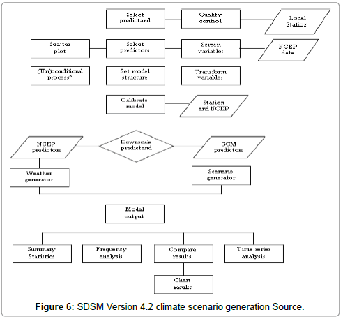
Figure 6: SDSM Version 4.2 climate scenario generation Source.
Model evaluation method
Four criteria were used to evaluate the model especially the generated output from the weather generator. These criteria are Coefficient of Determination (R2), Root Mean Square Error (RMSE), Mean Absolute Error (MAE) and Nash-Sutcliffe. Good agreement based on these criteria between the observed and generated data would be helpful for scenario generation; the calibration model assumes that relationship between the predictor and predictand under the current condition remain valid under future climate scenarios. Data analyses include:
Coefficient of determination: The coefficient of determination (R2) of a multiple linear regression model gives the proportion of the variances of the simulated data and observed data. Values closer to 1 show better fit of the model and better variation of the dependent variable can be explained by the independent variable. It is defined as:
 (5.2.1)
Where yi denotes the observed values of the predictand, y as the mean and  as the fitted/simulated value
Root Mean Square Error (RMSE): The Root Mean Square Error (RMSE) (also called the root mean square deviation, RMSD) is a frequently used measure of the difference between values predicted by a model and the values actually observed from the environment that is being modelled. These individual differences are also called residuals, and the RMSE serves to aggregate them into a single measure of predictive power. The RMSE of a model prediction with respect to the estimated variable Xmodel is defined as the square root of the mean squared error:
 (5.2.2)
Where Xobs is observed values and Xmodel is modelled values at time/place i
The RMSE values can be used to distinguish model performance in a calibration period with that of a validation period as well as to compare the individual model performance to that of other predictive models.
Mean Absolute Error (MAE): The Mean Absolute Error (MAE) is the difference of the absolute error of the generated/simulated data with the observed data. It also measures how close the simulated data into observed data. MAE is given by:
 (5.2.3)
Where yi denotes the observed values of the predictand, y as the mean and as the fitted/simulated value
Nash-Sutcliffe coefficient (E): The Nash-Sutcliffe model efficiency coefficient (E) is commonly used to assess the predictive power of hydrological discharge models. However, it can also be used to quantitatively describe the accuracy of model outputs for other things than discharge (such as nutrient loadings, temperature, concentrations etc.). It is defined as:
(5.2.4)
Where Xobs is observed values and Xmodel is modelled values at time/place i
Nash-Sutcliffe efficiencies can range from -∞ to 1. An efficiency of 1 (E=1) corresponds to a perfect match between model and observations. An efficiency of 0 indicates that the model predictions are as accurate as the mean of the observed data, whereas an efficiency less than zero (-∞<E<0) occurs when the observed mean is a better predictor than the model. Essentially, the closer the model efficiency to 1, the more accurate the model is.
Results and Discussion
Set of predictors were screened and chosen based on the correlation analysis between predictor and predictand variables over 12 months period at 95% level of confidence. These were carefully examined if identified predictors are conceptually and physically sensible at the local weather site. Table 1 shows high correlation of predictors vis a vis predictands of local weather station at Bago Oshiro, Agrometeorological Station. For temperature minimum (Tmin), eight (8) out of twenty six (26) predictors highly correlates with predictands, namely: p_z,p_th, p5_f, 850 hPa, p8th, s500, s850, and temp. For temperature maximum (Tmax), eight (8) out of twenty six (26) identified predictors which are highly sensible in downscaling temperature maximum; these are: slpg, p_th, p500, p5th, p5zh, s850, shum, temp. For precipitation, results shows seven (7) out of twenty six (26) predictors that correlate highly with predictors, namely: slpg, p u, p5_u, p500, p5zh, p8th, p8zh.
| Predictors Code | Description | Predictands | ||
|---|---|---|---|---|
| TMIN | TMAX | RAIN | ||
| slpg | Mean sea level pressure | X | X | |
| p__f | 1000 hPa Wind speed | |||
| p__u | 1000 hPa U-component | X | ||
| p__v | 1000 hPa V-component | |||
| p__z | 1000 hPaVorticity | X | ||
| p_th | 1000 hPa Wind direction | X | X | |
| p_zh | 1000 hPa Divergence | |||
| p5_f | 500 hPa Wind speed | X | ||
| p5_u | 500 hPa U-component | X | ||
| p5_v | 500 hPa V-component | |||
| p5_z | 500 hPaVorticity | |||
| p500 | 500 hPaGeopotential | X | X | |
| p5th | 500 hPa Wind direction | X | ||
| p5zh | 500 hPa Divergence | X | X | |
| p8_f | 850 hPa Wind speed | |||
| p8_u | 850 hPa U-component | |||
| p8_v | 850 hPa V-component | |||
| p8_z | 850 hPa Vorticity | |||
| p850 | 850 hPa Geopotential | X | ||
| p8th | 850 hPa Wind direction | X | X | |
| p8zh | 850 hPa Divergence | X | ||
| s500 | 500 hPa Specific humidity | X | ||
| s850 | 850 Specific humidity | X | X | |
| shum | 1000 hPa Specific humidity | X | ||
| temp | Temperature at 2m | X | X | |
| prcp | Accumulated precipitation | |||
Table 1: List of predictors from NCEP and CGCM3 datasets and selected predictors which highly correlates to each predictand.
Calibration and validation
Downscaling techniques is dependent upon the availability of data for model calibration and validation and the variables required for the assessment. The splitting of data sets follows the work of [28,29]; it encourages the use of cross validation and double cross validation of data in order to yield additional information. Since May 1976, the local weather station has gathered a total of 26 years weather data. For model calibration, it covers the period of 20 years (1976-1995) while, model validation covers 12 years (1989-2000). For calibration and validation figures, the line graph shows good agreement of the observed and simulated data of minimum and maximum temperature and precipitation. Tmin and Tmax figures show overlapping lines; some deviations of rainfall patterns are observed between the observed and simulated data. In general, the pattern and trend of the observed data is captured by the simulated data. Below are the figures illustrating the NCEP simulation and CGCM3 simulation performance of both calibration and validation? (Figures 7-12).
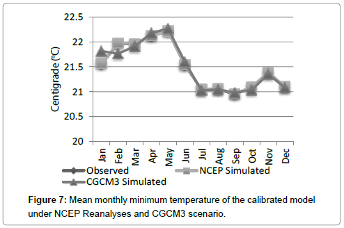
Figure 7: Mean monthly minimum temperature of the calibrated model under NCEP Reanalyses and CGCM3 scenario.
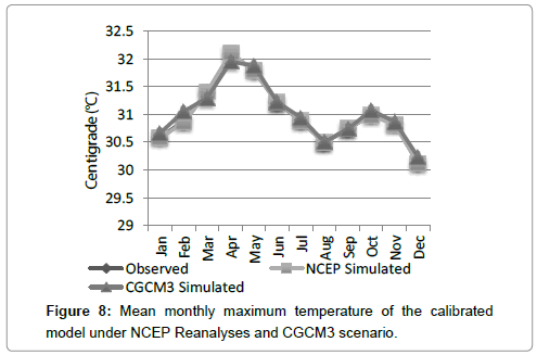
Figure 8: Mean monthly maximum temperature of the calibrated model under NCEP Reanalyses and CGCM3 scenario.
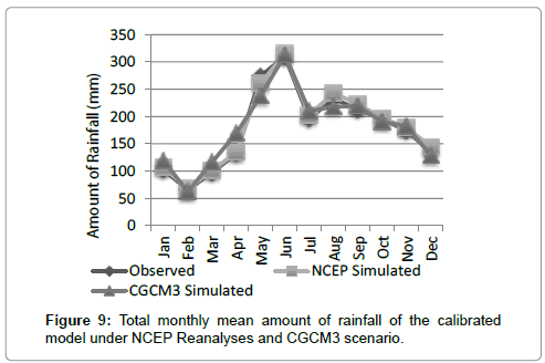
Figure 9: Total monthly mean amount of rainfall of the calibrated model under NCEP Reanalyses and CGCM3 scenario.
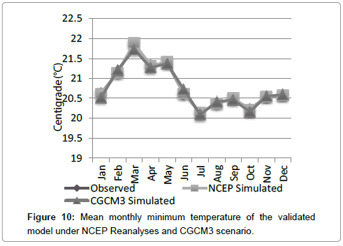
Figure 10: Mean monthly minimum temperature of the validated model under NCEP Reanalyses and CGCM3 scenario.
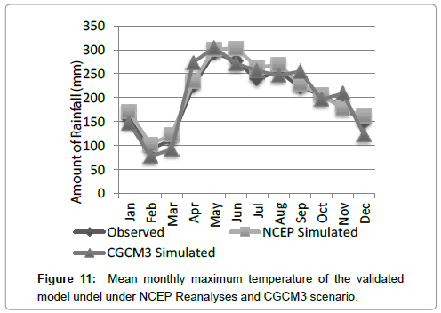
Figure 11: Mean monthly maximum temperature of the validated model undel under NCEP Reanalyses and CGCM3 scenario.
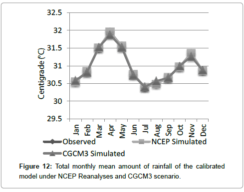
Figure 12: Total monthly mean amount of rainfall of the calibrated model under NCEP Reanalyses and CGCM3 scenario.
Table 2 illustrates the adequacy of the model as analysed using coefficient of determination; it also shows different values for each month during the calibration and validation under A1B and A2 scenarios. These variations can be attributed to the different parameters of the model created for each month. Different combinations of the predictors resulted to the different percentages on the variation of the model that can be explained by the independent variables (Table 3).
| Calibration | Validation | |||||
|---|---|---|---|---|---|---|
| RR | TMIN | TMAX | RR | TMIN | TMAX | |
| Jan | 0.7 | 18.12 | 32.94 | 22.07 | 43.6 | 12.78 |
| Feb | 30.27 | 24.38 | 28.83 | 27.11 | 33.14 | 67.34 |
| Mar | 6.17 | 27.13 | 9.39 | 68.64 | 53.53 | 0.1 |
| Apr | 0.54 | 46.48 | 42.8 | 42.69 | 20.69 | 3.57 |
| May | 9.85 | 29.91 | 27.82 | 17.74 | 5.85 | 62.34 |
| Jun | 35.2 | 15.06 | 30.05 | 9.46 | 37.09 | 55.14 |
| Jul | 1 | 16.85 | 16.64 | 18.28 | 0.94 | 71.08 |
| Aug | 53 | 37.25 | 6.29 | 16 | 53.72 | 43.75 |
| Sep | 12.33 | 43.39 | 42.41 | 37.5 | 26.32 | 16.02 |
| Oct | 29.28 | 32.79 | 0.41 | 11.91 | 22.2 | 8.63 |
| Nov | 0.77 | 39.19 | 22.74 | 22.06 | 64.17 | 28.22 |
| Dec | 38.08 | 33.73 | 35.11 | 52.79 | 59.94 | 32.02 |
Table 2: Monthly coefficient of determination for each predictand during the calibration and validation process under A1B scenario.
| RR | TMIN | TMAX | RR | TMIN | TMAX | |
|---|---|---|---|---|---|---|
| Calibration | Validation | |||||
| Jan | 11.29 | 27.61 | 1.63 | 0.79 | 19.64 | 43.5 |
| Feb | 18.41 | 32.09 | 61.33 | 53.04 | 28.96 | 49.35 |
| Mar | 4.47 | 18.3 | 1.86 | 2.88 | 46.74 | 0.82 |
| Apr | 18.45 | 35.1 | 1.74 | 40.76 | 28.53 | 85.69 |
| May | 6.57 | 31.27 | 0.85 | 4.2 | 57.18 | 0.28 |
| Jun | 40.22 | 25.37 | 20.63 | 11.42 | 47.43 | 26.6 |
| Jul | 14.96 | 47.34 | 16.05 | 30.38 | 5.34 | 39.97 |
| Aug | 28.42 | 16.62 | 14.24 | 30.24 | 71.72 | 47.64 |
| Sep | 14.77 | 48.2 | 25.15 | 35.21 | 35.39 | 54.31 |
| Oct | 1.39 | 44.58 | 7.78 | 0.95 | 19.74 | 47.43 |
| Nov | 10.45 | 22.54 | 9.26 | 34.66 | 69.28 | 47.06 |
| Dec | 2.4 | 33.57 | 20.92 | 42.19 | 61.77 | 42.25 |
Table 3: Monthly coefficient of determination for each predictand during the calibration and validation process under A2 scenario.
Minimal deviation between the observed data and the residual/ generated/simulated data resulted to better agreement. Computed RMSE and MAE were lower in minimum and maximum temperature compared to the rainfall during the calibration and validation processes under A1B and A2 scenarios (Tables 4 and 5).
| Calibration | Validation | |||||
|---|---|---|---|---|---|---|
| RR | TMIN | TMAX | RR | TMIN | TMAX | |
| RMSE | 12.99 | 1.57 | 1.29 | 14.97 | 1.62 | 1.47 |
| MAE | 7.49 | 1.18 | 0.93 | 8.38 | 1.13 | 1.05 |
| E | 0.003 | 0.0758 | 0.1316 | 0.0027 | 0.1224 | 0.1436 |
Table 4: Summarize model evaluation criteria under A1B scenarios.
| Calibration | Validation | |||||
|---|---|---|---|---|---|---|
| RR | TMIN | TMAX | RR | TMIN | TMAX | |
| RMSE | 13.12 | 1.57 | 1.32 | 14.81 | 1.62 | 1.49 |
| MAE | 7.57 | 1.17 | 0.96 | 8.32 | 1.16 | 1.07 |
| E | -0.02 | 0.085 | 0.09 | 0.024 | 0.122 | 0.121 |
Table 5: Summarize model evaluation criteria under A2 scenarios.
Downscaled station-scale climate projections
Temperature minimum: Climate Projections for temperature minimum are analyzed into three time slice periods:2020 (2011- 2040), 2050 (2041-2070) and 2080 (2071-2100) under two scenarios namely, A1B and A2 scenarios.A1B scenario shows minimal increase and decrease of the three time slice periods compared to observed data. Consistently, the month of March shows an increase in Tmin by 0.16°C and 0.24°C specifically for slice periods 2050 and 2080. It implies that for the month of March, Talomo-Lipadas Watersheds areas would experience higher temperature; consequently, higher temperature has a ripple effect to water-dependent communities, other living organisms, among others. Generally, for time slice period of 2020 (2011-2040) Tmin projection is observed to increase in the months of January, March, April, June, July, November, and December. In 2050 ( 2041-2070), Tmin is observed to increase significantly in the months of Feb, March, May, August, September, and October; the remaining months will have decreased temperature compared to observed data. In 2080, minimum temperature is observed to increase in the months of January, March, June, July, September, November, and December; the rest of the months will experience lower temperature. A2 Scenario shows erratic changes of minimum temperature. In 2020, the temperature is generally decreasing at most by 0.19°C compare to observed data. The general decrease in Tmin is the same in the time slice period, that is, 2050 and 2080 (Tables 6 and 7).
| OBS | A1B Scenario | A2 Scenario | |||||
|---|---|---|---|---|---|---|---|
| Centigrade (°C) | Centigrade (°C) | ||||||
| 2020 | 2050 | 2080 | 2020 | 2050 | 2080 | ||
| Jan | 21.39 | 0.05 | -0.65 | 0.05 | -0.89 | -0.09 | -0.70 |
| Feb | 21.78 | -0.37 | 0.37 | 0.00 | -0.46 | 0.00 | 0.28 |
| Mar | 22.14 | -0.05 | 0.72 | 1.08 | 0.14 | -0.09 | -0.59 |
| Apr | 21.93 | 0.09 | -0.96 | -0.55 | 0.27 | -0.14 | -0.23 |
| May | 22.05 | -0.45 | 0.09 | -0.23 | -0.50 | -0.63 | 0.45 |
| Jun | 21.38 | 0.33 | -0.14 | 0.00 | -0.19 | 0.37 | 0.19 |
| Jul | 20.89 | 0.10 | -0.14 | 0.10 | -0.38 | -0.14 | 0.10 |
| Aug | 21.07 | 0.05 | 0.14 | -0.05 | 0.33 | -0.52 | 0.19 |
| Sep | 21.09 | 0.00 | 0.52 | 0.00 | 0.05 | -0.05 | -0.09 |
| Oct | 21.07 | -0.47 | 0.00 | -0.09 | -0.19 | -0.43 | -0.52 |
| Nov | 21.39 | 0.05 | -0.75 | 0.05 | -0.89 | -0.05 | -0.14 |
| Dec | 21.21 | 0.47 | 0.00 | 0.71 | -0.52 | -0.71 | -0.33 |
Table 6: Percent change on projected minimum temperature under A1B and A2 scenario.
| OBS | A1B Scenario | A2 Scenario | |||||
|---|---|---|---|---|---|---|---|
| Centigrade (°C) | Centigrade (°C) | ||||||
| 2020 | 2050 | 2080 | 2020 | 2050 | 2080 | ||
| Jan | 30.57 | 0.56 | 0.13 | -0.39 | 0.33 | -0.33 | 0.23 |
| Feb | 30.86 | 0.06 | 0.13 | -0.16 | -0.39 | 0.00 | -0.29 |
| Mar | 31.49 | -0.38 | 0.44 | 0.13 | 0.16 | 0.35 | -0.10 |
| Apr | 32.06 | -0.37 | 0.03 | 0.06 | 0.22 | 0.25 | 0.28 |
| May | 31.65 | -0.22 | 0.09 | -0.06 | 0.19 | 0.00 | 0.32 |
| Jun | 30.94 | 0.16 | -0.10 | 0.42 | 0.10 | 0.32 | 0.23 |
| Jul | 30.57 | 0.33 | -0.10 | 0.13 | -0.16 | 0.39 | 0.29 |
| Aug | 30.45 | -0.10 | -0.16 | -0.03 | 0.00 | 0.16 | 0.03 |
| Sep | 30.63 | 0.07 | -0.03 | -0.20 | 0.00 | -0.20 | -0.07 |
| Oct | 30.94 | -0.10 | -0.10 | -0.26 | -0.03 | 0.19 | -0.19 |
| Nov | 31.11 | -0.06 | 0.16 | -0.06 | 0.26 | 0.03 | -0.03 |
| Dec | 30.56 | -0.13 | -0.20 | 0.23 | -0.56 | -0.36 | -0.36 |
Table 7: Percent change on projected maximum temperature under A1B and A2 scenario.
Comparatively, A1B scenario is hotter than A2 scenario. The result is confirmed by the study of Zemede Nigatu where among three scenarios (A1B, A2, and B2), A1B scenario has consistently higher increases in temperature compared to A2 and B2 scenario. Considering the minimal differences in increases/decreases, the months that showed to be hotter and wetter have subsequent implication to the climatedependent sectors especially among domestic water users, agricultural water users, and disaster (drought, landslide, and flashflood) disaster managers (Figures 13 and 14).
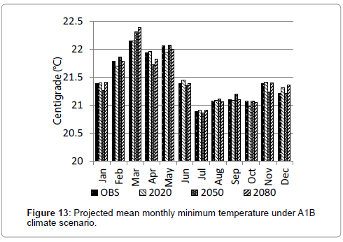
Figure 13: Projected mean monthly minimum temperature under A1B climate scenario.
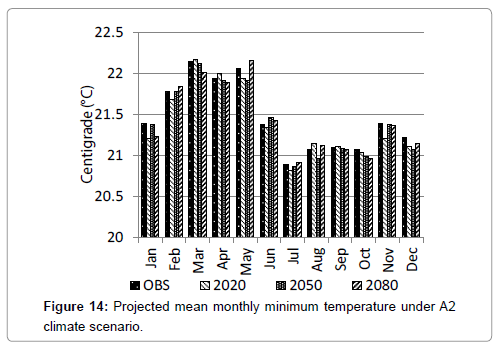
Figure 14: Projected mean monthly minimum temperature under A2 climate scenario.
Maximum temperature: Climate Projections are analyzed into three time slice periods: 2020 (2011-2040), 2050 (2041-2070) and 2080 (2071-2100) under two scenarios namely A1B and A2. From the observed data, for Tmax in A1B scenario, for time slice period of 2020, the months of January, February, June, July, and September will likely experience slightly hotter temperature compare to observed data; this means, both watersheds will become more drier than the normal Tmax ranges. The rest of the months will likely experience lower temperature. In time slice period of 2050, there is a slight increase of temperature for consecutive months starting from January, February, March, April, and May. This means a likely drought lasting for five months. Starting in the months of June until October, Tmax drops ranging -0.03 to -0.06. This is attributed to the fact that June is the start of rainy season. In time slice period of 2080, for Tmax in A1B scenario, March and April will likely become more hotter; interestingly this also include months of June and December. The rest of the months will experience minimal decrease of maximum temperature compared to observed maximum temperature. From the observed data, for Tmax in A2 scenario, for time slice period 2020, March and April are likely to experience intense temperature of 31.54 and 32.13°C, respectively. For slice time period of 2050, the watershed areas are likely to experience hotter and drier temperature with an increase of 0.12°C for the next thirty years. And this hotter and drier temperature is also observed for slice time period 2080 (Figures 15 and 16).
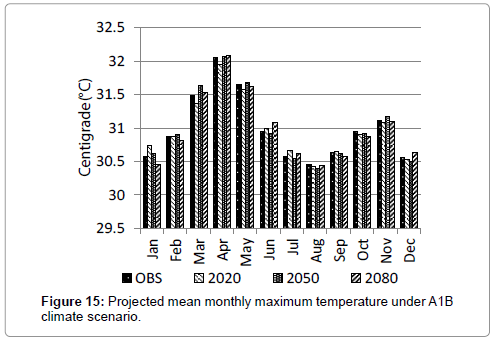
Figure 15: Projected mean monthly maximum temperature under A1B climate scenario.
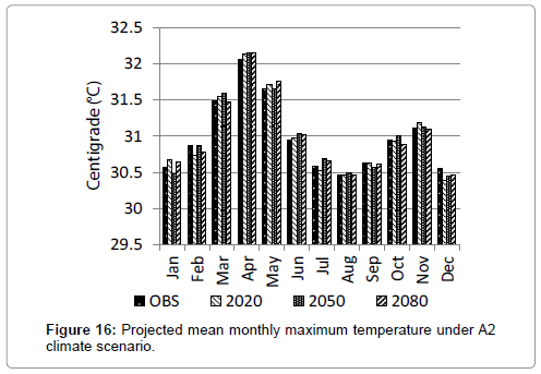
Figure 16: Projected mean monthly maximum temperature under A2 climate scenario.
Precipitation: Downscaled precipitation is analyzed into three time slice periods: 2020 (2011-2040), 2050 (2041-2070) and 2080 (2071- 2100) under two scenarios namely A1B and A2. For A1B Scenario and for slice time period of 2020, the months of January and April have climate scenario. an increase of 29.62% and 30.35% respectively. For 2050, the months of January, February, and March have an increase of 33.37%, 20.83% and 31.85% respectively. Notably, the time slice period of 2080 has the highest increase of 42.87% from the observed data of 81 to 116 mm for the month of February. For A2 Scenario, for three slice time periods of 2020, 2050 and 2080, the projected precipitation shows consistent and consecutive heavy rainfall with a remarkable increase in the months of January, February, and March. Evidently, in both scenarios, the findings show a wetter condition especially on the onset of the year (Table 8). This would imply more water to recharge in the aquifer. Apparently, the above findings, which are based on statistical downscaling method, deviated and contradicted PAG-ASA’s future projection which uses dynamical downscaling. Based on PAG-ASA’s report, no rainfall greater than 300 is projected for 2020 and 2050 under medium range emission (Climate Change in the Philippines, 2007 p42.). Statistical downscaling method has a projected of more than 300 mm specifically for the month of June (335 mm) under A2 scenario especially in the 2050 slice time period (Figures 17 and 18).
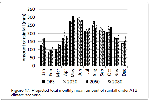
Figure 17: Projected total monthly mean amount of rainfall under A1B climate scenario.
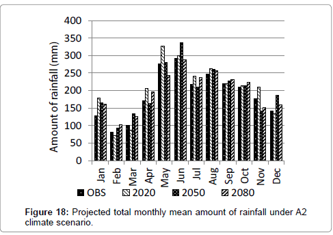
Figure 18: Projected total monthly mean amount of rainfall under A2 climate scenario.
| OBS | A1B Scenario | A2 Scenario | |||||
|---|---|---|---|---|---|---|---|
| (mm) | (mm) | ||||||
| 2020 | 2050 | 2080 | 2020 | 2050 | 2080 | ||
| Jan | 128 | 29.62 | 33.37 | -9.5 | 38.79 | 28.15 | 24.84 |
| Feb | 81 | 19.86 | 20.83 | 42.87 | -11.18 | 13.25 | 25.62 |
| Mar | 101 | -19.61 | 31.85 | 25.82 | -15.17 | 31.62 | 23.97 |
| Apr | 170 | 30.35 | -20.94 | 9.89 | 21.68 | -4.59 | 15.38 |
| May | 276 | 3.46 | 11.73 | 2.34 | 18.73 | 1.35 | -11.85 |
| Jun | 292 | 2.26 | -4.6 | -4.2 | 2.63 | 14.65 | -1.63 |
| Jul | 217 | 3.69 | -0.3 | 7.84 | 11.49 | -2.94 | 9.04 |
| Aug | 248 | 9.99 | -5.42 | 0.9 | 5.97 | 4.88 | 3.57 |
| Sep | 219 | 9 | 3.19 | -3.15 | -0.1 | 3.46 | 4.95 |
| Oct | 210 | 15.98 | 7.34 | 12.67 | 1.7 | 1.97 | 5.94 |
| Nov | 177 | -4.36 | -3.66 | 11.15 | 19.15 | -19.73 | -14.52 |
| Dec | 141 | -2.3 | 9.57 | 31.02 | -5.42 | 31.26 | 12.55 |
Table 8: Percent change on projected amount of rainfall under A1B and A2 scenario.
Conclusion
Projection of downscaled climate scenarios at station scale is becoming an indispensable tool in present time. It aids in formulating robust planned adaptation strategies, guides policy makers, water managers, and helps local communities to be more prepared in anticipating potential increases and decreases of climate variables like temperature and precipitation in coming years. For Talomo-Lipadas Watersheds, Davao City, Philippines, the downscaled temperature minimum (Tmin), is likely to increase of 0.16°C for time slice period of 2020 and 0.24°C in time slice period of 2080 in the month of March under A1B scenario. For temperature maximum (Tmax), generally, there is a likely slight increase compare to observed data both under A1B and A2 scenarios in all three time slice periods. Specifically for 2050 (2041-2070), five month long drought is likely to be experienced in the two watersheds. For precipitation; there is a significant increase in precipitation in the watershed areas especially in the onset of the year in both A1B and A2 scenarios in three slice time periods. Comparatively, A1B scenario is wetter than A2. Specifically, there is likely an increase of additional 42.87% from the observed data in the month of February in 2080 under A1B scenario. Notably, the month of June has the highest rainfall between 279-335 mm in both scenarios.
Acknowledgements
The authors are grateful to the financial support given by the University of Nairobi-IDRC Research Project Grants. Likewise, credits are due to the Commission on Higher Education (CHED) and to the University of Mindanao, Davao City, Philippines for the scholarship.
References
- UNFCCC (2005)Â Compendium on methods and tools to evaluate impacts of and vulnerability and adaptation to climate change.
- Wilby RL, Dawson CW, Barrow EM (2001)SDSM — a decision support tool for the assessment of regional climate change impacts. J Environ Model Softw 17: 145–157.
- Adaptayo (2011) Climate Change in the Philippines. Climate Projections in the Philippines, Joint project of MDGF.
- Climate Change (2007) Synthesis Report: An Assessment of the Intergovernmental Panel on Climate Change.
- Cohen SJ (1990) Bringing the global warming issue closer to home: the challenge of regional impact studies. Bull Am Met Soc 71: 520-526.
- Gates WL (1985) The use of general circulation models inthe analysis of the ecosystem impacts of climatic change. Clim Change 7: 267-284.
- Lamb PJ (1987) On the development of regional climatic scenarios for policy-oriented climatic-impact assessment. Bull Am Met Soc 68: 1116-1123.
- Robinson PJ, Finkelstein PL (1989) Strategies for Development of Climate Scenarios. Final Report to the U.S. Environmental Protection Agency. Atmosphere Research and Exposure Assessment Laboratory, Office of Research and Development, USEPA, Research Triangle Park, NC, 73.
- Smith JB, Tirpak DA (1989) The Potential Effects of Global Climate Change on the United States.Report to Congress, United States Environmental Protection Agency, Washington, DC.
- Hostetler S (1994) Hydrologic and atmospheric models: the problem of discordant scales: an editorial comment. Clim Change 27: 345-350
- Carter TR, Parry ML, Harasawa H, Nishioka S (1994) IPCC Technical Guidelines for Assessing Climate Change Impacts and Adaptations: part of the IPCC special report to the first session of the conference of the parties to the UN framework convention on climatic change. Department of geography, University college of London.
- DAI CGCM3 Predictors (2008)Sets of Predictor Variables Derived From CGCM3 T47 and NCEP/NCAR Reanalysis Montreal, QC, Canada.
- Klein WH, Glahn HR (1974) Forecasting local weather by meansof model output statistics. Bull Am Meteorol Soc 55: 1217–1227.
- Carter TR, Hulme M, Lal M (1999) Guidelines on the Use of Scenario data for Climate Impact and Adaptation Assessment. Intergovernmental Panel on Climate Change. Task Group on Scenarios for Climate Impact Assessment 69.
- Mearns LO, Giorgi F, Pabon WD, Hulme M, Lal M (2003)Â Guidelines for Use of Climate Scenarios Developed from Regional Climate Model Experiments. DDC of IPCC TGCIA.
- Wilby RL, Dawson C (2007) SDSM - A decision support tool for the assessment of regional climate change impacts. J environ model softw 17: 145-157.
- IPCC (1996)Â Climate change 1995: The Science of Climate Change. Contribution of Working Group I to the Second Assessment Report of the Intergovernmental Panel on Climate Change. Houghton JT, MeiraFilho LG, Callander BA, Harris N, Kattenberg A,MaskellK (edn)], Cambridge University Press, Cambridge 572.
- Alila Y, Beckers J (2001) Using numerical modelling to address hydrologic forest management issues in British Columbia. Hydrol Process 15: 3371–3387
- Hillel D (1986) Modeling in soil physics: A critical review, InFuture developments in soil science research. Soil Science Society of America, Madison, WI.
- Leaf CF (1975) Watershed management in the Rocky Subalpine zone: The status of our knowledge. USDA Forest Service Research paper RM 137: 28-31.
- US Environmental Protection Agency (1980) An approach to water resources evaluation on non-point silvicultural sources (a procedural handbook). United States Environmental Protection Agency, Environmental Research laboratory, Athens.
- Measham TG, Preston BL, Smith TF, Brooke C, Gorddard R, et al. (2011) Adapting to climate change through local municipal planning: barriers and challenges. Mitigation and Adaptation Strategies for Global Change 16: 889-909.
- Adger WN, Kelly PM (1999) Social vulnerability to climate change and the architecture of entitlements. Mitig Adapt Strateg Glob Change 4:253-266.
- Cutter SL, Mitchell JT, Scott MS (2000) Revealing the vulnerability of people and places: a case study of Georgetown County, South Carolina. Ann Assoc Am Geogr 90:713-737.
- Turner BL, Kasperson RE, Matson PA, McCarthy JJ, Corell RW, et al. (2003) A framework for vulnerability analysis in sustainability science. ProcNatlAcadSci USA 100:8074-8079.
- Abdel-Fattah SL (2012)Downscaling the GreatLakes: Techniques for Adaptive Policy. Open Access Dissertations and Theses Paper 7435.
- Kozak A, Kozak R (2003)Does cross validation provide additional information in the evaluation of regression models? Canadian J forest res 33: 976-987.
Citation: Branzuela NE, Faderogao FJF, Pulhin JM (2015) Downscaled Projected Climate Scenario of Talomo-Lipadas Watershed, Davao City, Philippines. J Earth Sci Clim Change 6: 268. DOI: 10.4172/2157-7617.1000268
Copyright: ©2015 Branzuela NE, et al. This is an open-access article distributed under the terms of the Creative Commons Attribution License, which permits unrestricted use, distribution, and reproduction in any medium, provided the original author and source are credited.
Select your language of interest to view the total content in your interested language
Share This Article
Recommended Journals
Open Access Journals
Article Tools
Article Usage
- Total views: 16728
- [From(publication date): 3-2015 - Jul 17, 2025]
- Breakdown by view type
- HTML page views: 11997
- PDF downloads: 4731