Modelling Atmospheric Concentrations of Particulate Matter Model Climate Sensitivity of Ecosystems and Feedbacks for Region South Algeria

This paper has three main goals:

• To introduce the physical basis and the mathematical description of the different components of the climate system and the derivation of differential equations which describe the most important climatic processes,

• To introduce in the numerical solutions of ordinary partial differential equations using examples from climate modelling;

• To use and apply Matlab as a mathematical-numerical tool. In this work the predictability of atmospheric flow depends on the current state of the atmosphere. Predictability can be determined by integrating an ensemble of initial conditions that are within certain predefined bounds. We employ the software package Matlab for the numerical simulations in this paper. The feasibility and effectiveness of the proposed method is demonstrated by computer simulation. Some wildlife species require large stretches of land in order to meet all of their needs for food, habitat, and other resources. These animals are called area sensitive. When the environment is fragmented, the large patches of habitat no longer exist. It becomes more difficult for the wildlife to get the resources they to survive, possibly becoming threatened or endangered. While environmental degradation is most commonly associated with the activities of humans, the fact is that environments are also constantly changing over time. With or without the impact of human activities, some ecosystems degrade over time to the point where they cannot support the life that is “meant” to live there.

The modelling of the scattering of the pollutants in the atmosphere is based on the resolution of an equation to the partial derivatives that binds the temporal evolution of the concentration in one point to the phenomena of diffusion and transportation in the atmosphere, the concentration of air pollutants in the atmosphere is directly linked to air quality. High ground level air pollution concentration can affect both the public’s health and the environment. There are regulations in many countries that require the applicant to do an air dispersion modelling in order to obtain an approval certificate for building a new facility. Dispersion models can be used to predict the cumulative effect of existing and planned facilities. In order to predict Ground Level Concentration (GLC) from various sources, atmospheric dispersion models are essential. In the setting of the modelling of the scattering of the pollutants in the atmosphere it remains to try to solve the equation diffusion-transportation bound to the concentrations of pollutants only. To solve this equation various possibilities offer themselves based: - on an algebraic approach, and a numeric approach.

In a first time we have, as makes usually for reasons of calculation capacity, privileged the algebraic method.

This method consists in replacing the equation to the partial derivatives that conditions the distribution of the concentrations by an algebraic equation in which one takes into account the phenomena physics of diffusion and transportation through the intermediary of coefficients bound downwind to the distance, the stability and to the conditions of broadcasts to the air atmosphere. The method Gaussian is based on the hypothesis of the stationeries. To introduce in the numerical solutions of ordinary partial differential equations using examples from climate modelling; and to use and apply Matlab as a mathematical-numerical tool.

Atmospheric dispersion modeling refers to the mathematical description of contaminant transport in the atmosphere, physical and chemical processes have to be described by mathematical terms in the beginning of the development of a continental air pollution model. These processes are: horizontal transport (advection), horizontal diffusion, chemical transformations in the atmosphere combined with emissions from different sources, deposition of pollutants to the surface, and vertical exchange (containing both vertical transport and vertical diffusion). The dispersion models are used to estimate or to predict the downwind concentration of air pollutants or toxins emitted from sources such as industrial plants, vehicular traffic or accidental chemical releases. The partial differential equation to be solved is the classical advection dispersion equation extended with source sink terms to account for the sorption and degradation processes; the advectiondiffusion equation reduces to

            (1)

The height difference between the virtual source and the real source is called the plume height. Due to the transient conditions in which the particles is liberated to the atmosphere, and being the dispersion a three-dimensional phenomenon, transient results of concentration are generated for a fixed height plane of interest (z).

The elevation phenomenon occurs as a function of wind velocity. Consider the numerical solution of the advection - dispersion equation assuming that D=0. In this case there is only advection without any physical dispersion/diffusion

                                         (2)

Explicit finite difference approximation for

                                         (3)

Where sub index i refers to node and sub-index n to time (n+1 unknown value and n known).

The unknown concentration at time level n+1 can be solved from

                                         (4)

Otherwise R is a nonlinear function of the solute concentration C.

Equations (1-3), and (3-4) are solved numerically using the finite difference method (Figure 1).

Advection, diffusion and convection

In nature the transport of energy and tracers is determined by three processes: advection, diffusion and convection. These three processes induce fluxes of matter and energy, of which the mathematical description is derived by continuum mechanics. Advection is caused by a flow which transports matter and energy. Diffusion is a random process taking place at all times and leading to a net transport only under certain conditions. Convection occurs where instabilities in fluid or gaseous systems exist. Such instabilities themselves cause secondary circulations and finally modifications of the large-scale flows.

Approaches numerical

The main objective of this work is to calculate the condition of dispersion and diffusion of pollutants en atmosphere for case in south Algeria. We consider again the climate model given by equation (2) but we examine its time dependence. It is clear that an analytical solution is only possible for few cases. For this reason, it has to be solved using a numerical algorithm. Several types of analytical solutions exist for the transport/sorption/degradation problem but they are limited to some special cases. However, analytical solutions are very useful tools to verify the accuracy of the numerical solution methods and test the correctness of a computer program. Elliptic PDE’s are equations with second derivatives in space and no time derivative. The most important examples are Laplace’s equation, the formulations assume an equidistant discretization; adjustments are necessary if the grid’s resolution is spatially dependent, is the numerical solution (5-10) and Figures 1-4, consistent with the analytical solution; either to solve the hyperbolic system:

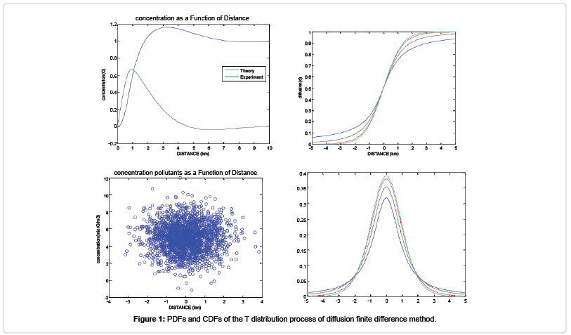
Figure 1: PDFs and CDFs of the T distribution process of diffusion finite difference method.

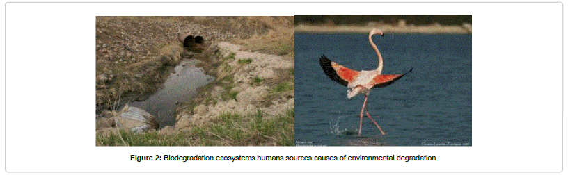
Figure 2: Biodegradation ecosystems humans sources causes of environmental degradation.

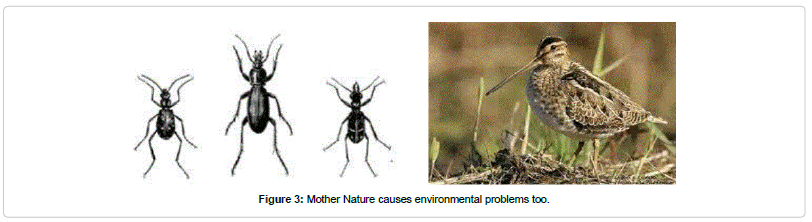
Figure 3: Mother Nature causes environmental problems too.

Figure 4: The solution of 3D transport in the space (x) – time (t) diagram, visualized.

                                         (5)

we didn’t suppose here the conservation of the sign of the characteristic k_i(x,t) speed

                                         (6)

Either (x,t) a point of grid we write the equations to the differentials that correspond to him; so k_i (x, t)

Therefore we apply a transformation of variables,

     (7)

If k_i(x, t) > 0

Using central difference in space, and forward difference in time we get

     (8)

u_i(x,t) the exact solution of the equations to the partial derivatives that of the derivatives first and seconds according to the formula of Taylor

     (9)

Hence, it has been shown that the numerical solution converges towards the analytical solution

for arbitrarily small Δt

            (10)

This is a distinctive feature of the equation to be solved. Central differences may also cause general problems in the case, for example, that periodic solutions with unluckily chosen time steps should be calculated (Figures 2 and 3).

That we have an error-free computer program, it will predict only what it has been designed to do and that is, the model can make predictions about a system based only upon the assumptions in the model. In the case of modelling.

Wild populations or ecosystems, it is imperative that the modeler spend time in the natural system to observe its components and their relationships. This Simulation was conducted in MATLAB environment and the results are presented for the case of three sources configuration, in work of [1-5], we’ve considered a single source in a constant wind. To solve the 2-D governing Euler equations a code was developed in this work, with the software MATLAB 7.8.version using the Jameson’s scheme, which is a finite volume spatial discretization method with artificial dissipative term. We still need to include: Multiple sources (still with constant emission rate), Time-dependent wind velocity, not aligned with x-axis, multiple contaminants. Ultimately, solve the inverse problem.

The Matlab code used to produce (Figures 4-6) is given below. The Matlab code used to solve equation (3-6) and equation 7-10 analytically and numerically, and plot Figures 5 and 6 is given below. The chemical reaction equations were solved simultaneously with the governing equations of transport reaction diffusion in horizontal dispersion. Any numerical scheme exhibits non-physical properties due to the truncation. By neglecting high-order terms in the Taylor expansion, errors are introduced. Numerical diffusion is one of them and it becomes particularly obvious when the real diffusion of physical properties needs to be quantified (Figures 4-8).

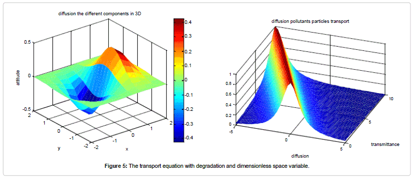
Figure 5: The transport equation with degradation and dimensionless space variable.

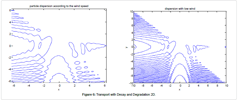
Figure 6: Transport with Decay and Degradation 2D.

Figure 7: 5 D- mapping a geographic area south Algeria.

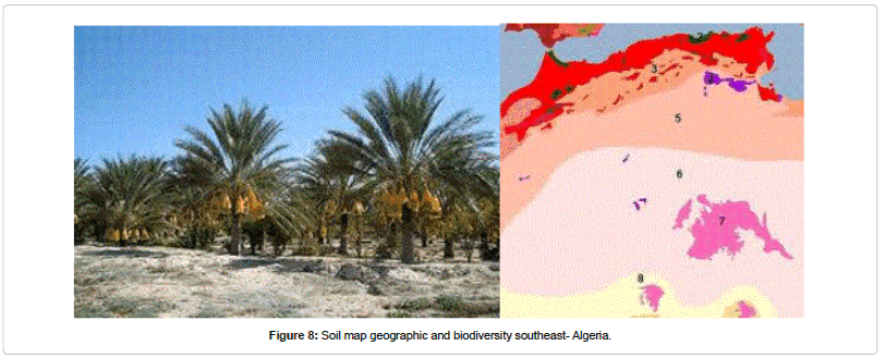
Figure 8: Soil map geographic and biodiversity southeast- Algeria.

The effects of land pollution can be found everywhere. Pollutants in the land not only contaminate the land itself, but also have far-reaching consequences. There are a number of reasons those ecosystems (Figures 7 and 8), degrade over time. While it may not always be the fault of humans, humans still need to recognize the extent to which they rely on the resources that the natural world provides. In this sense, environmental responsibility and stewardship are very much a matter of self-preservation, and are an integral part of healthy resource management practices.

In this paper, we have provided a detailed look at the basic mathematics behind atmospheric dispersion modelling, based on Gaussian plume approximations to the advection–diffusion equation with a continuous point source. When land pollution is bad enough, it damages the soil. This means that plants may fail to grow there, robbing the eco-system of a food source for animals. Eco-systems may also be upset by pollution when the soil fails to sustain native plants, but can still support other vegetation. Invasive weeds that choke off the remaining sources of native vegetation can spring up in areas that have been weakened by pollution. This Simulation was conducted in MATLAB environment and the results are presented for the case of three sources configuration, in work of references [1,6-8] we’ve considered a single source in a constant wind. We still need to include: Multiple sources (still with constant emission rate), Time-dependent wind velocity, not aligned with x-axis, multiple contaminants. Ultimately, solve the invers problem. The suggested numerical solution method for combined advection, dispersion/diffusion and Biodegradation gives very accurate results when compared to analytical solutions. Many of the long-lasting effects of land pollution, such as the leaching of chemicals into the soil cannot be easily reversed. The best way to deal with land pollution is to keep it from happening in the first place. A further important motivation for the development and application of climate models remains the aim to assess future climate change.

References

- Huckabee JW, Goldstein RA, Janzen SA, Woock SE(1977) Methylmercury in a Freshwater Foodchain. In International Conference on Heavy Metals in the Environment, Toronto, Ontario, Canada.
- Holzbecher E (1998)Modeling Density-Driven Flow in Porous Media. Springer Publishing,Heidelberg, Germany.
- Holzbecher E (2002) Groundwater Modeling-Simulation of Groundwater Flow and Pollution, FiatLux Publishing, Fremont, USA.
- Hornberger G,Wiberg P (2005) Numerical Methods in Hydrological Sciences. Am Geophys Union Washington DC, USA.
- Jared S (2014) Causes of Environmental Degradation. BA Environmental Science, USA.
- BiswalDK, Kumar V,Barik K (2012) Dispersion Modeling of Jaipur Fire, India. Res J Chem Sci 2: 1-9.
- Zlatev Z, Christensen J,Eliassen A (1993) Studying high ozone concentrations by using the Danish Eulerian Model.Atm Environ 27: 845-865.
- Dixon KR(1977) Thermal Plumes and Mercury Dynamics in Zooplankton. In International Conference on Heavy Metals in the Environment, Toronto, Ontario, Canada.
Citation: Ferhat M (2014) Modelling Atmospheric Concentrations of Particulate Matter Model Climate Sensitivity of Ecosystems and Feedbacks for Region South Algeria. J Earth Sci Climat Change S11: 005. DOI: 10.4172/2157-7617.S11-005
Copyright: © 2014 Ferhat M. This is an open-access article distributed under the terms of the Creative Commons Attribution License, which permits unrestricted use, distribution, and reproduction in any medium, provided the original author and source are credited.
Select your language of interest to view the total content in your interested language
Share This Article
Recommended Journals
Open Access Journals
Article Tools
Article Usage
- Total views: 15272
- [From(publication date): 0-2014 - Jul 01, 2025]
- Breakdown by view type
- HTML page views: 10626
- PDF downloads: 4646