Optimum Pattern and Rate Injection Determination of Waterflooding Project (Case Study in Block "A" on "DS" Field)
Received: 06-Apr-2019 / Accepted Date: 19-Apr-2019 / Published Date: 26-Apr-2019 DOI: 10.4172/2472-0518.1000166
Abstract
“DS” field is one of the mature field located in Block “A” which has been produced since 1975. The remaining reserves of this field is 14,285 MSTB with remaining recovery factor 25.04%. The Water Oil Contact is up-leveling during the production phase where in current condition, this field has high water cut which means high water production. While the remaining reserves is still big enough to produce and the field produces a lot of water, field development with waterflooding method may be applied. Analysis of development scenarios using ECLIPSE 2010.1 reservoir simulation software. The parameter considered is the pattern and rate of injection. Base case is a scenario that simulates the field from history matching condition until August 2032. Scenario 2 with peripheral injection pattern and the 9 scenarios of injection rate. Scenario 3 with regular injection patterns 5 and 6 spots injection rate scenario. Scenario 4 with regular injection patterns 4 spot and 6 injection rate scenario. From engineering analysis, the best scenario is Scenario 2 with 10 peripheral injection wells but from economic analysis, the best fit scenario is Scenario 3 with 8 5-spot injection wells.
Keywords: Reservoir simulation; Waterflooding; Pattern; Injection rate; Development scenario
Introduction
“DS” field is located in the Central Sumatra Basin, Sumatra, Indonesia. The number of wells currently active (until December 2011) is 27 wells. Until December 2011, there are 36 wells on the “DS” field with 27 production wells that still produce with primary recovery method, 4 abandoned wells, and 5 suspended wells. “DS” field is one of the mature fields that has been produced since 1975. There was a decrease in the field rate of production measured in 2009-2013 from 1,000 BOPD to 600 BOPD. The remaining reserves at this field is 14,285 MSTB which is big enough to be produce trough seconderay recovery method.
Since “DS” field has a high water production (high water cut), large remaining reserves and able to utilize a large water production, then thisfield is considered to be developed with waterflooding methods.
The purpose of this paper is to develop Field “DS” to waterflooding methods to improve oil recovery in the field “DS”. Meanwhile, the objective is to determine the pattern of injection and optimum injection rate that can be applied to the field “DS” [1].
Material and Methods
Here are the steps being taken to solve the problems in the paper are: Collecting and processing the necessary data, specifying drainage radius wells are then made bubble map, Determining candidates injection wells, injection wells Determining patterns. Determining the injection rate, doing scenario development to determine the pattern and the optimum injection rate; and evaluate the scenario by incremental RF, RF parameters, and economic analysis [2]. The methodology of this paper is shown in Figure 1.

Figure 1: Methodology of “DS” Field Development.
According to Thakur, Ganesh. in the development of waterflooding, there are some things that need to be considered in planning the development of the flood pattern waterflooding among other things, performance prediction, and determination of reserves [2].
Water injection is a water injection rate per unit pressure difference between the production and injection wells. A drastic decline in water injection occurs at the beginning of the injection until the reservoir is filled solution gas drive. After the fill-up, variations of water injection rate is also affected by the mobility ratio. If M=0 then it will be a constant injection rate, increased if M>1 (which is not expected), and decreased if M<1 (which is expected). Criteria for a court to say the prospect of doing waterflooding is a field that has a high water cut and the field have an adequate water supply injection [3]. Stages in the development field “DS” using waterflooding as follows:
Specifying drainage radius and plotted on the bubble map
The radius of the absorption is the radial distance from a borehole in the reservoir where there is fluid flow (oil and water) into the well and outside the boundary where the pressure reservoir fixed and no fluid flow occurs. The radius of the intended absorption is effective draining radius (re) to each well which has not changed and is the maximum value of the radius of dewatering wells (rd) at steady state conditions [4].
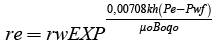 (1)
(1)
where; re: boundary radius, ft; Pwf: bottom-hole flowing pressure, psi; rw: well radius, ft; mo: oil viscosity, cp; k: permeability, mD; Bo: oil formation volume factor, bbl/STB; h: thick of layer, ft; qo: rate of oil production, bbl.day; Pe: external boundary pressure, psi.
After getting the calculation of drainage radius of each well, then be plotted on the bubble map.
Determining candidates injection wells
In the Field development “DS” to waterflooding methods, candidate wells - injection wells are used to suspend the conversion wells and production wells are analyzed using the scatter plot by watching the water parameters and cumulative high cut low production and small production rate [5].
Determining the injection pattern
Injection pattern is one important parameter in planning waterflooding. Pattern - a pattern that can be applied include direct line, regular and inverted 4 spots, 5 spots, 7 spots, 9 spots, peripherals.
These are the images of injection pattern according to Ganesh Thakur and Wilhite (Figures 2-7) [1].

Figure 2: Injection Direct Line Pattern.

Figure 3: Injection Pattern 4 Spot.

Figure 4: Pattern Injection 5 Spot.

Figure 5: Pattern Injection 7 Spot.

Figure 6: Injection Pattern 9 Spot

Figure 7: Injection 10 Spot Pattern.
Injection rate determination
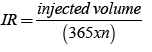
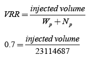
The Injection rate is determined by the method of voidage replacement ratio. Voidage Replacement Ratio (VRR) is the ratio of the volume of fluid injection with a fluid volume of production (Aldousary, 2015). Mathematically expressed in eqns. (2) and (3).
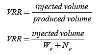 (2)
(2)
 (3)
(3)
where;
Wp: cumulative water production (MBBL); Np: cumulative oil production (MBBL); IR: the rate of water injection (bbl/day); N: time of injection (days).
Scenario analysis results against rf
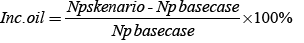
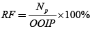
The parameters that determine the effectiveness of development scenarios performed on Field “DS” to calculate the increase and incremental oil recovery factor from each scenario against basecase. Eqn. (4) shows the RF equation and eqn. (5) shows the determination of incremental oil equation [6].
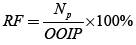 (4)
(4)
 (5)
(5)
where; RF: Recovery Factor, %; Inc. oil: Incremental Oil to the Basecase, %.
Case Study
Data
The reservoir on “DS” Field located on two formation: Layer A with 50 ft of thickness and Layer B with 150 ft of thickness. Productive formation of “DS” field is shown in Figure 8 and Table 1.

Figure 8: Productive Formation of “DS” Field.
| Parameter | Information |
|---|---|
| OOIP | 49,488 MSTB |
| Backup Time | 14,285 MSTB |
| Drive Mechanism | Water Drive |
| RF | 25.04% |
| API Gravity Oil | 31.7 |
| Initial Pressure | 2,860 psi |
Table 1: Data Reservoir and Simulation.
Determination drainage radius depletion
The drainage radius draining manually calculated by eqn. (1). Example calculation of the drainage radius of DS_1 wells. Field drainage radius “DS” on the Layer A is shown in Figure 9. Radius dewatering and Field “DS” on the Layer B is shown in Figure 10.

Figure 9: Re Field “DS” Layer A.

Figure 10: Field Re “DS” Layer B.
Determination of injection wells
Prospects of production wells used injection wells are wells that have had high water cut and low Np. Figure 11 shows the results of the analysis of the scatter plot of water cut Cumulative (%) with cumulative oil production (bbl) in the Field “DS” [7]. The classifications are shown in Table 2.

Figure 11: Scatter Plot Candidates Injection Wells.
| Class | Water Cut (%) | Np (Mbbl) | Oil Rate (bbl/day) |
|---|---|---|---|
| High | >95.4 | >816 | >26 |
| Medium | 89.6-95.4 | 235.5-816 | 11.0-26 |
| Low | <89.6 | <235.4 | <11 |
Table 2: Classification of Injection Well Based on Water Cut, Np, and Oil Rate.
In addition to notice water cut and cumulative production parameters, determining candidate also noticed parameter injection wells oil production rate. based on analysis of the ability of the reservoir, obtained the following classifications. Table 3 shows the results of the analysis of the injection wells candidate determination based oil rate.
| Well | Oil Rate (bbl/day) | Information |
|---|---|---|
| DS_11 | 8 | LOW |
| DS_12 | 10 | LOW |
| DS_14 | 0 | LOW |
| DS_15 | 0 | LOW |
| DS_16 | 0 | LOW |
| DS_18 | 0 | LOW |
| DS_23 | 0 | LOW |
| DS_24 | 8 | LOW |
| DS_11 | 8 | LOW |
| DS_12 | 10 | LOW |
| DS_5 | 8 | LOW |
| DS_26 | 4 | LOW |
| DS_28 | 3 | LOW |
| DS_29 | 8 | LOW |
| DS_30 | 8 | LOW |
| DS_34 | 8 | LOW |
| DS_35 | 5 | LOW |
Table 3: Determination of Wells Injection Candidate Analysis.
Injection pattern determination
Based on the analysis of the determination of the injection wells, there are 17 wells that are candidates injection wells. The number of production wells, there were 15 wells. In consideration of injection wells more of the production wells injection patterns that can be applied is peripheral, regular 5 spot, and regular 4 spot. Third injection pattern will be divided into three development scenarios. In scenario 1 with peripheral injection patterns, there are 10 injection wells. Producing wells in the Field “DS” as many as 22 wells. Figure 12 shows the injection patterns in scenario 2. Table 4 shows the tabulation of the injection wells and production wells scenario 2.

Figure 12: Pattern of Peripheral Injection Scenario 2.
| Injection wells | Location Grid |
|---|---|
| DS_8 | B1 |
| DS_7 | C2 |
| DS_18 | A4 |
| DS_17 | A5 |
| DS_15 | A6 |
| DS_16 | C8 |
| DS_29 | E8 |
| DS_14 | A7 |
| DS_9 | C7 |
| DS_26 | B6 |
Table 4: Well Injection - Production Scenario.
Table 5 shows the tabulation of injection and production wells in Scenario 3 with regular injection patterns 5 spot. Injection pattern in Scenario 3 is shown in Figure 13.

Figure 13: Pattern of Peripheral Injection Scenario 3.
| Production | Injection |
|---|---|
| DS_20 | DS_11, DS_26, DS_15, DS_30 |
| DS_31 | DS_24, DS_9, DS_16, DS_29 |
Table 5: Injection wells - Production Scenario 3.
Table 6 shows the tabulation of injection and production wells in scenario 4 with a regular injection patterns 4 spot. Patterns injection in scenario 4 is shown in Figure 14.
| Production wells | Injection wells |
|---|---|
| DS_3 | DS_34, DS_35, DS_23 |
| DS_27 | DS_5, DS_18, DS_17 |
| DS_31 | DS_24, DS_9, DS_29 |
| DS_32 | DS_30, DS_9, DS_15 |
Table 6: Well Injection - Production Scenario 4.

Figure 14: Pattern of Peripheral Injection Scenario 4.
Injection rate determination
Field “DS” has never been the development of the field with waterflooding methods, then there is no data prior injection rate. The injection rate is determined by the method of voidage replacement ratio [8]. The amount of injection rate calculated by eqns. (2) and (3).
Injected Volume = 16,180,281 Mbbl/year
N (days) = 1/02/2018 - 7/31/2032 (5294 days)
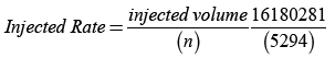
Injected Rate = 3,300 bbl/day
Scenario development
There are several scenarios performed on Field “DS”, among others: Scenario 1 (Bas ecase): In basecase, the predictions made by forwarding the production wells that are still in production (27 wells) at the end of history matching up to August 2032.
Scenario 2 (Basecase+conversion of 10 wells): In this scenario made the development of the basecase+conversion of 10 production wells into injection wells, which means there are 17 production wells. In this scenario conducted some sensitivity rate of up to optimum such as 330 bbl/day, 500 bbl/day, 800 bbl/day, 1000 barrels/day, 2000 barrels/day, 2500 barrels/day, 10000 bbl/day, 15000 bbl/day, and 20000 bbl/day. This scenario made on February 1, 2018 until July 2032. The pattern of injection wells is peripheral (Table 7).
| Case | Objectives | Notes |
|---|---|---|
| Scenario 1 (BC) | Do nothing | Production from 27 existing wells |
| Scenario 2 | Basecase + Conversion of 10 Wells – Peripheral (17 Production Wells) | Rate Sensitivity: |
| 2A. 330 bbl/day | ||
| 2B. 500 bbl/day | ||
| 2C. 800 bbl/day | ||
| 2D. 1,000 bbl/day | ||
| 2E. 2,000 bbl/day | ||
| 2F. 2,500 bbl/day | ||
| 2G. 10,000 bbl/day | ||
| 2H. 15,000 bbl/day | ||
| 2I. 20,000 bbl/day | ||
| Scenario 3 | Basecase + Conversion of 8 Wells - Regular 5 Spot (19 Production Wells) | Rate Sensitivity: |
| 3A. 412 bbl/day | ||
| 3B. 500 bbl/day | ||
| 3C. 800 bbl/day | ||
| 3D. 1,000 bbl/day | ||
| 3E. 2,000 bbl/day | ||
| 3F. 2,500 bbl/day | ||
| Scenario 4 | Basecase + Conversion of 11 Wells - Regular 4 Spot (16 Production Wells) | Rate Sensitivity: |
| 4A. 253 bbl/day | ||
| 4B. 500 bbl/day | ||
| 4C. 800 bbl/day | ||
| 4D. 1,000 bbl/day | ||
| 4E. 2,000 bbl/day | ||
| 4F. 2,500 bbl/day |
Table 7: Scenarios for Field Development.
Scenario 3 (Basecase+Conversion of 8 wells): In this scenario do development basecase+conversion of 8 wells into the injection wells, which means there are 19 production wells. In this scenario conducted some sensitivity rate of up to optimum such as 412 bbl/day, 500 bbl/ day, 800 bbl/day, 1000 barrels/day, 2000 barrels/day, and 2500 bbl/day. Skenario was conducted on February 1, 2018 to July 2032. The pattern of injection wells is a regular 5 spot.
Scenario 4 (Basecase+conversion of 11 wells): In this scenario made the development of the basecase+conversion of 11 production wells into injection wells, which means there are 16 production wells. In this scenario conducted some sensitivity rate of up to optimum such as 253 bbl/day, 500 bbl/day, 800 bbl/day, 1000 barrels/day, 2000 barrels/day, and 2500 bbl/day. This scenario made on February 1, 2018 until July 2032. The pattern of injection wells is a regular 4 spot.
Result
Scenario 1 (Basecase, 27 production wells)
Basecase is to maintain the last state scenario Field “DS” which consists of 27 production wells were simulated by the end of 2032. The results of prediction basecase used as a basis of comparison in the next scenario planning so they will know the amount of the increase in oil recovery and recovery factor. At the end of 2032 with the existing wells, 27 production wells are obtained cumulative oil production amounted to 13,764,277 STB and RF 27.81%. The recovery factor in the Field “DS” decrease from the original 38.92% to 27.81% due to more wells were dead because of pitch-cut off by contraints on basecase. With this scenario, field able to produce until August 2032. RF calculations were done using eqn. (4) (Figure 15).

Figure 15: Results Injection Rate Basecase Courses.
 (6)
(6)
Scenario 2 (Basecase+conversion of 10 wells)
In scenario 2 with peripheral injection patterns performed 9 injection rate scenarios [9]. All injection wells whether new or existing, are assumed to cost USD 600,000/well/year. The cost of installation of the water injection pump, for example, an Elmar water/grease. The cost of installing a gathering system for the water gathering and maintenance is USD 100,000. The cost of installing water lines for transporting the water from the oil well where the water well is, execution of associated civil works and maintenance of water facility for two years is less than USD 950,000. So, the total cost for injection plant is USD 85,050,000. Table 8 shows the results of the injection rate scenario in scenario 2.
| Sken. | Rate (bbl/day) | NP (STB) | RF (%) | Incr. (%) |
|---|---|---|---|---|
| 2A | 330 | 1,44,03,380 | 29.1 | 1.291 |
| 2B | 500 | 1,44,16,182 | 29.13 | 1.317 |
| 2C | 800 | 1,44,37,587 | 29.17 | 1.361 |
| 2D | 1,000 | 1,44,51,079 | 29.2 | 1.388 |
| 2E | 2,000 | 1,45,09,753 | 29.32 | 1.506 |
| 2F | 2,500 | 1,45,34,246 | 29.36 | 1.556 |
| 2G | 10,000 | 1,47,45,824 | 29.79 | 1.983 |
| 2H | 15,000 | 1,47,81,505 | 29.86 | 2.056 |
| 2I | 20,000 | 1,47,38,987 | 29.78 | 1.97 |
Table 8: RF Tabulation and Incemental Oil on Skenario 2.
Determining the optimum rate is not indicated by the acquisition of the largest cumulative oil production but by determining the intersections between it and injection rate [10]. Thiss well able to produce until August 2032. The result of the analysis of the optimum injection rate shown in Figure 16.

Figure 16: Rate Analysis Optimum Scenario 2.
In scenario 2 with the peripheral injection pattern optimum injection rate of 6,600 bbl/day with 14,640 Mbbl of oil cumulative production. With this scenario, field able to produce until August 2032 with 2,865 bbl/day of oil production rate. By assuming that production cost is 5 USD/bbl, then total production cost is 73,200,000 USD .
Scenario 3 (Basecase+conversion of 8 wells)
In scenario 3 with regular injection patterns performed 5 spot injection rate scenario [9].
All injection wells whether new or existing, are assumed to cost USD 600,000/well. The cost of installation of the water injection pump, for example, an Elmar water/grease. The cost of installing a gathering system for the water gathering and maintenance is USD 100,000. The cost of installing water lines for transporting the water from the oil well where the water well is, execution of associated civil works and maintenance of water facility for two years is less than USD 950,000. So, the total cost for injection plant is USD 68,250,000. Table 9 shows the results of injection rate scenarios in Scenario 3.
| Sken. | Rate (bbl/day) | Np (STB) | RF (%) | Incr. (%) |
|---|---|---|---|---|
| 3A | 412 | 1,43,24,782 | 28.946 | 1.133 |
| 3B | 500 | 1,43,39,391 | 28.975 | 1.162 |
| 3C | 800 | 1,43,85,445 | 29.069 | 1.255 |
| 3D | 1,000 | 1,44,07,337 | 29.113 | 1.299 |
| 3E | 2,000 | 1,44,54,031 | 29.207 | 1.394 |
| 3F | 2,500 | 1,44,52,390 | 29.204 | 1.39 |
Table 9: RF Tabulation and Incemental Oil on Skenario 3.
Determining the optimum rate is not indicated by the acquisition of the largest cumulative oil production but by determining the intersections between injection rate and Np [9]. Results of analysis of optimum injection rate shown in Figure 17.

Figure 17: Rate Analysis Optimum Scenario 3.
In scenario 3 with the peripheral injection pattern optimum injection rate of 1,270 bbl/day with 14,420 Mbbl of oil cumulative production. With this scenario, field able to produce until August 2032 with 2,822 bbl/day of oil production rate. By assuming that production cost is 5 USD/bbl, then total production cost is 72,100,000 USD.
Scenario 4 (Basecase+conversion of 11 wells)
In scenario 4 with regular injection patterns performed 4 spot injection rate scenario (Ahmad Tarek, 2012).
All injection wells whether new or existing, are assumed to cost USD 600,000/well. The cost of installation of the water injection pump, for example, an Elmar water/grease. The cost of installing a gathering system for the water gathering and maintenance is USD 100,000. The cost of installing water lines for transporting the water from the oil well where the water well is, execution of associated civil works and maintenance of water facility for two years is less than USD 950,000. So, the total cost for injection plant is USD 93,450,000. Table 10 shows the results of injection rate scenarios in Scenario 4 with the acquisition of Np.
| Sken. | Rate (bbl/day) | Np (STB) | RF (%) | Incremental (%) |
|---|---|---|---|---|
| 4A | 253 | 1,41,24,848 | 28.54 | 0.729 |
| 4B | 500 | 1,41,69,838 | 28.63 | 0.82 |
| 4C | 800 | 1,42,15,517 | 28.72 | 0.912 |
| 4D | 1,000 | 1,42,35,542 | 28.76 | 0.952 |
| 4E | 2,000 | 1,42,69,069 | 28.83 | 1.02 |
| 4F | 2,500 | 1,42,42,892 | 28.78 | 0.967 |
Table 10: RF Tabulation and Incemental Oil on Skenario 4.
Determining the optimum rate is not indicated by the acquisition of the largest cumulative oil production but by determining the intersections between injection rate and Np [11]. Results of analysis of the optimum injection rate shown in Figure 18.

Figure 18: Rate Analysis Optimum Scenario 4.
Table 11 showed the analysis of optimum injection rate for the whole scenario. In scenario 4, with the peripheral injection pattern optimum injection rate of 1,150 bbl/day with 14,240 Mbbl of oil cumulative production. With this scenario, field able to produce until August 2032 with 2,822 bbl/day of oil production rate. By assuming that production cost is 5 USD/bbl, then total production cost is 71,200,000 USD (Figure 18) .
| Scenario | Inj. Rate (bbl/day) | Np (Mbbl) | % RF | % Inc RF |
|---|---|---|---|---|
| 2 (peripheral) | 6,600 | 14,640 | 29.58 | 1.77 |
| 3 (regular 5 spots) | 1,270 | 14,420 | 29.13 | 0.96 |
| 4 (regular 4 spots) | 1,150 | 14,240 | 28.77 | 1.32 |
Table 11: Tabulation Injection Rate Optimum Whole Scenario.
Economic analysis
The selection of the best scenario wasn’t only analyzed based on the increase of cumulative oil production and recovery factor obtained from each scenario [12]. However, it is important to consider the economics of each scenario. Table 12 shows production cost estimation; Table 13 shows injection plant cost estimation; and Table 14 shows cost analysis of “DS” field.
| Scen | Prod. Wells | Q, (bbl/day) | Production Cost (USD/bbl) | Total Production Cost (USD) |
|---|---|---|---|---|
| 2 | 17 | 2,865 | 5 | 7,32,00,000 |
| 3 | 19 | 2,822 | 5 | 7,21,00,000 |
| 4 | 16 | 2,787 | 5 | 7,12,00,000 |
Table 12: Total Production Cost of “DS” Field.
| Scen. | Injc. Wells | Inj. Cost (USD/well) | Maint. & Gath. System (USD) |
|---|---|---|---|
| 2 | 10 | 6,00,000 | 1,00,000 |
| 3 | 8 | 6,00,000 | 1,00,000 |
| 4 | 11 | 6,00,000 | 1,00,000 |
| Scen. | Water Plant (USD) | Total Injection Cost (USD) | |
| 2 | 9,50,000 | 8,50,50,000 | |
| 3 | 9,50,000 | 6,82,50,000 | |
| 4 | 9,50,000 | 9,34,50,000 | |
Table 13: Total Injection Cost of “DS” Field.
| Scen. | Total Production Cost (USD) | Total Injection Cost (USD) | Gross Income (Np x 50 USD/bbl, USD) | Net Income (USD) |
|---|---|---|---|---|
| 2 | 7,32,00,000 | 8,50,50,000 | 87,84,00,000 | 72,01,50,000 |
| 3 | 7,21,00,000 | 6,82,50,000 | 86,52,00,000 | 72,48,50,000 |
| 4 | 7,12,00,000 | 9,34,50,000 | 85,44,00,000 | 68,97,50,000 |
Table 14: Cost Analysis of “DS” Field.
Based on the economic analysis above, each scenario produces different profits according to the treatment in each scenario.
Discussion
Field “DS” is an old oil field located in Block A, Central Sumatra Basin, Indonesia. The decline of the rate production at Field “DS” occur at the year 2009-2013 is from 1,000 BOPD to 600 BOPD. The productive zone of “DS” field is located at Bekasap Sihapas Group Formation. The condition of the reservoir consists of 120°F reservoir temperature and 438 ft of datum depth reservoir. From the laboratory result, the API of the oil is 31.29, the viscosity is 23.9686 cp, and the dominant composition of hydrocarbon is C7+ (87.6%).
Based on the analysis of the scatter plot, there are 16 production wells into injection wells among other candidates DS_14, DS_15, DS_16, DS_18, DS_23, DS_28, DS_26, DS_35, DS_29, DS_24, DS_32, DS_34, DS_12, DS_30, DS_37, and DS_17. Moreover, PI matching done at the key well and some of the production wells that still alive such as DS_31, DS_32, DS_33, DS_36.
Injection patterns which can be applied to the field “DS” is peripheral, regular 5 spot, and regular 4 spot with more consideration of wells into injection wells compared to a production well. This is based on the total injection wells which are 17 wells and total production wells which is 15 wells.
Voidage Replacement Ratio Based on the analysis, the optimum injection rate of Field “DS” is based on an analysis of 3300 bbl/day. This method is the comparison between the injected volume fluids with the total fluids being produced [13-15].
There are 22 development scenarios performed on Field “DS”. Based on the engineering analysis of reservoir simulation conducted obtained Np (cumulative production) and RF (recovery factor), scenario optimum that can be applied to the field “DS” is the injection pattern of peripherals of 10 injection wells with the injection rate of 6,600 bbl/day which resulted in the acquisition of Np at 14,640 MSTB, RF 29.58%. But economically speaking, the best scenario for this field is Scenario 3 with 8 5-spot injection wells since it has the highest net income on 72,850,000 USD. This is because the operational cost for 8 injection wells is cheaper than operation cost for 10 injection wells compare to income achieved from the oil cumulative production from both scenarios [16-18].
Conclusion
1. Based on the analysis of the scatter plot, there are 16 production wells into injection wells among other candidates DS_14, DS_15, DS_16, DS_18, DS_23, DS_28, DS_26, DS_35, DS_29, DS_24, DS_32, DS_34, DS_12, DS_30, DS_37, and DS_17.
2. Injection patterns which can be applied to the field “DS” is peripheral, regular 5 spot, and regular 4 spot with more consideration of wells into injection wells compared to a production well.
3. Voidage Replacement Ratio Based on the analysis, the optimum injection rate of Field “DS” is based on an analysis of 3,300 bbl/ day.
4. From engineering analysis, the best scenario is Scenario 2 with 10 peripheral injection wells but from economic analysis, the best fit scenario is Scenario 3.
Acknwoledgement
The author would like to thank Petroleum Engineering Department of UPN “Veteran” Yogyakarta for supporting this research.
References
- Ganesh CT, Satter A (1994) Integrated Petroleum Reservoir Management. Chapter Terms, pp: 103-105.
- Ali E, Rintu K, Salwa MAH, Rahima AA, Henri FJ, et al. (2011) Waterflood Conformace Control in Heavy Oil, Multilayer Reservoir. IPTC. Bangkok. Thailand.
- Alvarez J, Ronald PS, Raul M (2014) Heavy Oil waterflooding: Back to the future. SPE Heavy and Extra Heavy Oil Conference. Colombia.
- Archer JS, Wall CG (1986) Petroleum Engineering priciples and Practice. Graham and Trotmand. London, United Kingdom, Chapter 11, pp: 173-183.
- Awotunde AA, Najmudeen S (2012) Consideration of Voidage Replacement Ratio in Well Placement Optimization. SPE Kuwait International Petroleum Conference and Exhibtion. Kuwait.
- Dennis B (2008) Waterflooding Viscous Oil Reservoirs. Indian Oil and Gas Technical Conference and Exhibition.
- Bradley WB (2008) Increasing Oil Recovery from Heavy Oil Waterfloods. SPE International Thermal Operations and Heavy Oil Symposium. Canada.
- Donaldson, Erle C (1985) Enhanced Oil Recovery. Elsevier Science Publishing Company INC. New York. Chapter 8, pp: 251-273.
- Gonzales L, Jose F, Mac F, Nerio C, Edison G, et al. (2014) Use of Reservoir Simulation to Estimate Drainage Area and Recovery Factor of an In-Situ Combustion Project in a Complex Water Drive Reservoir. SPE Heavy Oil Confrence. Canada.
- Hanafy HH, Mansy AM (1999) Waterflooding of A Marginal Heavy Oil Reservoir. Middle East Oil Show Presentation. Bahrain.
- Dedy K, Rukmana D (2011) "Reservoir Engineering Theory and Applications". Printing the Tree of Light. Yogyakarta. Chapter VIII, p: 232.
- Rosario O, Hernandez JCF, Korabelnikov AI (2017) Analytical Method for Voidage Replacement Ratio Calculation in Reservoir with Quasicritical Fluid. SPE Annual Technical Conference and Exhibition. Texas. USA.
- Smith GE (1992) Waterflooding Heavy Oils. SPE Rocky Mountain Regional Meeting. Casper. Wyoming.
- Thakur GC (2012) Heavy Oil Reservoir Management. SPE Fifth Latin American and Caribbean Petroleum Engineering Conference and Exhibition. Rio de Janerio, Brazil.
- Thomas CE (1962) Petroleum Engineering Handbook. Core Laboratories Inc. Houston, USA, Chapter 44, p: 1.
- Steven V (2011) Optimal Voidage Replacement Ratio for waterflood Communicating Heavy Oil Wells. SPE Heavy Oil Conference and Exhibition. Kuwait.
- Vittoratos SE (2013) VRR<1 is Optimal for Heavy Oil Waterfloods . SPE Offshore Europe Oil & Gas Conference and Exhibition. UK.
- Willhite GP, Waterflooding. SPE Foundation. United States. Chapter 6, pp: 199-224.
Citation: Herianto (2019) Optimum Pattern and Rate Injection Determination of Waterflooding Project (Case Study in Block “A” on “DS” Field). Oil Gas Res 5: 166. DOI: 10.4172/2472-0518.1000166
Copyright: © 2019 Herianto. This is an open-access article distributed under the terms of the Creative Commons Attribution License, which permits unrestricted use, distribution, and reproduction in any medium, provided the original author and source are credited.
Select your language of interest to view the total content in your interested language
Share This Article
Recommended Journals
Open Access Journals
Article Tools
Article Usage
- Total views: 6227
- [From(publication date): 0-2019 - Dec 11, 2025]
- Breakdown by view type
- HTML page views: 5238
- PDF downloads: 989