Journal of Earth Science & Climatic Change
Open Access

Sediment rating curve (SRC), Machine learning, Seasonal variation, Suspended sediment load, Hydrological modeling, Mahakali River Basin, SVM, KNN, Random Forest

Introduction

Nepal’s river systems are diverse and complex, shaped by the country’s dramatic topography and seasonal monsoon climate. These rivers are broadly categorized into three groups based on their origin and hydrological behaviour: major Himalayan rivers such as the Koshi, Gandaki, Karnali, and Mahakali, which are fed by glaciers and snowmelt and remain perennial with consistent dry-season flow (Chaulagain (2009)); medium rivers like the Babai, Bagmati, and Kankai, originating from the Mahabharat Range, relying on a mix of rainfall and groundwater with notable seasonal variability; and smaller Terai rivers draining the Siwalik Range, which are largely seasonal and require storage infrastructure for sustained use (Shrestha et al. (2011)) (Talchabhadel et al. (2021)). This classification reflects not only physical differences but also distinct hydrological responses influenced by Nepal’s varied climatic zones, from high- altitude glacial catchments with rapid runoff to lowland areas with greater groundwater influence (Khadka et al. (2020)). These river systems are influenced by rugged topography and a distinct monsoonal climate, exhibit highly variable hydrological and sediment transport dynamics. Understanding these patterns is essential for effective water resource management, particularly in the context of sediment load estimation (WECS (2011)) (Chinnasamy et al. (2020)). Sediment transport is driven by high erosion rates, glacial melt, and intense monsoon rainfall. These factors result in elevated suspended sediment concentrations during the monsoon season (Andermann et al. (2012)) (Chhetri et al. (2016)). Sediment is transported through traction, saltation, suspension, and solution, influencing river morphology and ecosystem health (Benda et al. (1997)). While sediment is essential for nutrient cycling and habitat maintenance, excessive loads can degrade water quality, harm aquatic life, and challenge infrastructure like hydropower plants (Chitrakar et al. (2019)). Understanding sediment dynamics is crucial for sustainable river management in the region.

Rating curves are commonly used hydrological tools that establish empirical relationships between river discharge and variables such as stage height or sediment concentration. These curves are typically developed using regression models fitted to historical field data (Tfwala et al. (2016)). They are especially valuable for estimating sediment loads in rivers where direct measurements are limited by logistical, financial, or safety constraints, particularly during high- flow events such as floods (Horowitz (2003)) (Thomas (1985)). However, conventional rating curves often fail to fully capture the complex, non-linear behavior of sediment transport, which can be influenced by hysteresis effects and changes in sediment availability under varying flow conditions (Tfwala et al. (2016)) (Boukhrissa et al. (2013)). In practice, sediment rating curves generally exhibit a curvilinear shape, with steep slopes at low flows that gradually flatten at higher discharges (Ponce (2023)).

Machine learning (ML) has emerged as a powerful and increasingly indispensable tool in hydrological research, particularly for improving the accuracy of sediment rating curve (SRC) models. The growing availability of high- resolution hydrological data from field sensors, remote sensing platforms, and long-term monitoring systems has enabled the application of data-driven techniques to complex hydrological processes. Traditional SRC methods, which rely on empirical regression approaches, often struggle to capture the nonlinear and time-dependent relationships between river discharge and suspended sediment concentration (Van et al. (2023)) (Nda et al. (2023)) (Atieh et al. (2015)). These limitations are especially pronounced in regions with dynamic hydrological behavior, such as Nepal, where factors like steep topography, seasonal monsoon variability, and glacial melt contribute to highly variable sediment transport patterns. ML algorithms such as Artificial Neural Networks (ANNs), Support Vector Machines (SVMs), and Random Forests offer a more flexible and adaptive approach by identifying hidden patterns in large datasets and modeling complex, nonlinear interactions without requiring explicit process-based equations (Lund et al. (2022)) (Jamal Chachan et al. (2022)) (Boukhrissa et al. (2013)). Studies have shown that ML based SRC models outperform conventional methods in terms of predictive accuracy, as demonstrated by improved performance metrics (Baniya et al. (2019)). Furthermore, ML models can better account for hysteresis effects and temporal shifts in sediment availability, which are common during monsoon-driven high-flow events. Given the critical role of accurate sediment load estimation in water resource planning, reservoir management, and hydropower operations, integrating ML into SRC development offers a promising pathway toward more robust and adaptive sediment management strategies in Nepal’s diverse and climatically sensitive river basins (Maharjan et al. (2024)) (Shrestha et al. (2011)). Due the complex nature of sediment and technical constrain in measurement; Nepal’s river basin has very few recordings of sediment data. This study tries to develop the SRC for Mahakali River Basin (MRB) (Station Number 120) using historical data of discharge and suspended sediment recorded by Department of Hydrology and Meteorology (DHM) using three different ML techniques; K-Nearest Neighbors (KNN), Support Vector Machines (SVM) and Random Forest (RF).

2.Material and Methodology

The primary data source for this study consists of suspended sediment and discharge measurements recorded by the Department of Hydrology and Meteorology (DHM) at station number

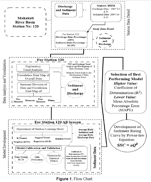
120 in MRB from 2007 to 2014. Analysis of the dataset reveals that while discharge data were available for 100% of the study period, sediment data were significantly incomplete, with only 30.49% temporal coverage over the same decade. This discrepancy in data availability presents a major challenge for effective river basin planning and management. To address this limitation and enable more accurate sediment load estimation, this study was designed to develop a predictive model for suspended sediment concentration based on the readily available discharge data. Following Figure 1 explains the detail process of study.

2.1 Mahalaki River Basin

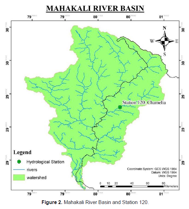
The Mahakali River forms the natural western boundary between Nepal and India along much of its course before entering Indian territory at the Lakhimpur Kheri district of Uttar Pradesh. It is a transboundary river of significant hydrological and geopolitical importance. The exact origin of the Mahakali remains a subject of dispute: Nepal asserts that the river’s true source lies at Limpiyadhura, where the longer tributary emerges, while India maintains that the river originates from the Lipulekh Glacier. This divergence in source identification reflects broader bilateral sensitivities regarding water rights and territorial delineation (Tiwari et al. (2025)) (Figure 1).

Figure 1: Flow Chart.

The Mahakali River basin spans a total area of 15,260 km² up to the Upper Sharda Barrage, with approximately 34% of this area located in Nepal (WECS (2005)). At the Lower Sharda Barrage, the total catchment expands to 19,243 km², of which the Nepal portion (NPB) accounts for 5,548 km² and the Indian portion (IPB) covers 13,695 km² comprising 10,871 km² in Uttarakhand and 2,824 km² in Uttar Pradesh. The basin traverses diverse topographic and climatic zones, originating in the high Himalayas and flowing southward through rugged mountainous terrain into the Siwalik Hills and the Terai plains (WECS (2005)).

In Nepal, the basin encompasses the districts of Darchula, Baitadi, Dadeldhura, and Kanchanpur in Sudurpaschim Province. On the Indian side, it covers Pithoragarh, Bageshwar, Champawat, and parts of Almora, Nainital, and Udham Singh Nagar districts in Uttarakhand, as well as Lakhimpur Kheri, Shahjahanpur, and Pilibhit districts in Uttar Pradesh. Rapid urbanization has been observed in recent years, particularly in Kanchanpur (Nepal) and various urban centers in Uttarakhand and Uttar Pradesh, increasing pressure on water resources and land use patterns within the basin.

The Mahakali River is perennial, fed by a combination of monsoon rainfall, snowmelt, and glacial sources, resulting in high seasonal discharge variability. It plays a critical role in regional water resource management, supporting irrigation, hydropower generation, and domestic water supply on both sides of the border (Tiwari et al. (2025)). However, high sediment loads due to steep slopes, fragile geology, and intense monsoon rains pose significant challenges for infrastructure sustainability, particularly in proposed and existing hydropower projects. Despite its importance, long- term and consistent sediment monitoring remains

limited, necessitating robust modeling approaches for sediment load estimation (WECS (2011)). This study focuses on Station No. 120 Chamelia River (figure 2) in the Nepalese part of the basin, leveraging available hydrological data to improve sediment rating curve development through machine learning techniques (Figure 2).

Figure 2: Mahakali River Basin and Station 120.

2.2 Discharge and Sediment Data Processing

The discharge and sediment trend analysis serve as a foundational component in understanding the hydrological behavior and sediment transport dynamics at Station No. 120 within MRB. The study begins with an evaluation of the frequency distribution of daily discharge (FDC), which provides valuable insights into the river’s flow regime. This analysis highlights distinct seasonal patterns, including pronounced peak flows during the monsoon season and significantly reduced flows during the dry period. Concurrently, temporal trends in suspended sediment concentration are examined to assess how sediment transport responds to variations in discharge over time. Given that discharge data were available for the entire study period (2007–2014), while sediment data were limited and irregularly sampled, a key step in the research involved developing a consistent daily sediment dataset. To overcome this data scarcity, average daily sediment values were generated from the available observations using statistical aggregation and interpolation methods. Subsequently, both discharge and sediment datasets were processed to obtain daily averaged values, ensuring temporal alignment and consistency between the two variables. These synchronized daily average datasets were then utilized as the primary input for model development, facilitating a more accurate and reliable representation of the discharge sediment relationship under varying hydrological conditions.

To enhance data consistency and remove anomalies, outlier detection and removal were performed using the 1.5 × Inter-Quartile Range (IQR) rule. Under this method, any data point lying beyond 1.5 times the IQR above the third quartile (Q3) or below the first quartile (Q1) was classified as an outlier and excluded from the analysis (Aggarwal (2017)). Finally, the cleaned and aggregated dataset was partitioned into training and testing subsets, with 80% of the data allocated for model training and the remaining 20% reserved for performance evaluation (Hyndman et al., 2006). This split ensured robust model validation while preserving the temporal structure of the data.

2.3 Seasonal Variation and its Importance in SRC

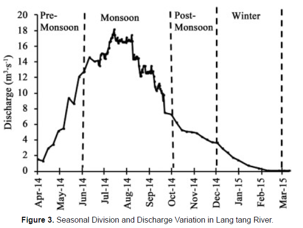
Nepal’s river systems exhibit pronounced seasonal variations in both discharge and sediment transport, driven by the country’s distinct monsoon climate and complex topography. The hydrological year is typically divided into four main seasons, pre- monsoon (April- June), monsoon (June–October), and post-monsoon (October- December) and winter (December–March) as shown in figure 3 suggested by (Chhetri et al. (2016)) in their research paper Assessment of Sediment Load of Langtang River in Rasuwa District, Nepal. These each season is characterized by unique flow and sediment dynamics (WECS (2011)). During the monsoon season, intense rainfall and accelerated glacial melt lead to peak discharges and sediment loads, with studies indicating that up to 80% of annual flow and over 80% of total sediment transport occur during this period (WECS (2011)) (Chhetri et al. (2016)) (Andermann et al. (2012)). In contrast, the pre-monsoon season sees moderate increases in flow due to snowmelt, while the post-monsoon and winter months are marked by significantly reduced flows and minimal sediment transport (Chhetri et al. (2016)). These seasonal shifts not only influence the magnitude of sediment load but also affect the relationship between discharge and suspended sediment concentration (SSC), with varying correlation strengths observed across seasons (Chhetri et al. (2016)). Notably, hysteresis effects: where sediment concentrations differ for the same discharge level at different times are more pronounced during the monsoon, complicating the development of accurate sediment rating curves (SRCs) (Chhetri et al. (2016)) (Morin et al. (2018)). Understanding these seasonal patterns is therefore essential for improving SRC modeling, as traditional regression-based approaches often fail to capture the nonlinear and time-dependent behaviour of sediment transport. Incorporating seasonal variability into SRC development enhances predictive accuracy, particularly in data-scarce regions like Nepal, where reliable sediment estimation is critical for effective water resource management, hydropower planning, and flood risk mitigation (Figure 3).

Figure 3: Seasonal Division and Discharge Variation in Lang tang River.

2.4 Need for Machine Learning in Sediment Rating Curve (SRC) Development and Justification for Model Selection

Sediment rating curves (SRCs) are essential tools for estimating suspended sediment load (SSL) in river systems, typically based on the empirical relationship between river discharge and sediment concentration. However, traditional SRC methods often derived using linear method struggle to capture the complex, nonlinear, and temporally dynamic interactions that govern sediment transport. These limitations become particularly pronounced under variable flow conditions, seasonal shifts, and high-flow events such as monsoon floods, where hysteresis effects, sediment availability, and antecedent moisture conditions significantly influence the discharge sediment relationship (Ponce (2023)) (Walling et al., 1988). As a result, conventional approaches tend to underestimate SSL, especially during peak flows, leading to potential inaccuracies in sediment budgeting, reservoir siltation assessments, and infrastructure planning.

To overcome these challenges, machine learning (ML) techniques have emerged as powerful alternatives, offering data-driven modeling capabilities that can better represent the non-linear and time-dependent behavior of sediment transport processes. Among various ML models, K-Nearest Neighbors (KNN), Support Vector Machines (SVM), and Random Forest (RF) have demonstrated particular relevance and effectiveness in SSL estimation. Each model brings unique strengths and limitations, but their comparative performance and adaptability to hydrological applications justify their use over traditional methods.

The K-Nearest Neighbors (KNN) algorithm is a non-parametric, instance-based method that estimates SSL by identifying similar historical discharge sediment patterns within the dataset. Its simplicity and ability to detect local trends make it useful for preliminary modeling, particularly in basins with relatively stable hydrological behavior (Ezzaouini et al. (2022)).

The Support Vector Machine (SVM) model excels at handling non-linear relationships through kernel functions, which project input data into higher-dimensional spaces for improved classification or regression performance. This makes SVM particularly effective in modeling complex sediment transport dynamics influenced by multiple variables such as rainfall, temperature, and land use. (Azamathulla et al. (2010)) reported R² of 0.958, and the mean square error, 0.0698, of the SVM method are higher than those of the traditional method for SSL prediction in Muda, Langat, and Kurau rivers.

Random Forest (RF) has consistently demonstrated superior performance in SSL prediction due to its ensemble nature, which combines multiple decision trees to reduce variance and improve generalization. RF excels in capturing non- linear interactions among predictors and is inherently resistant to overfitting, making it ideal for modeling sediment transport under varying climatic and hydrological conditions. Studies by (Ezzaouini et al. (2022)) from Morocco’s Bouregreg Basin showed that RF achieved Nash–Schiff efficiency (NSE) values of 0.47 to 0.80 during the validation phase, indicating satisfactory performances in predicting SSL.

Given the complex, nonlinear relationship between sediment concentration and discharge, particularly under varying hydrological conditions and the proven effectiveness of machine learning models in capturing such dynamics, the selection of KNN, SVM, and RF was based on their demonstrated performance in previous sediment load prediction studies. These models are well-suited for uncovering hidden patterns and interactions within hydrological datasets that traditional methods often fail to represent accurately. Their ability to handle non-linear dependencies, manage high- dimensional input spaces, and generalize across different flow regimes makes them particularly appropriate for developing a robust sediment rating curve (SRC) for Station No. 120 in the Mahakali River Basin.

2.5Model Parameter Tuning

a) KNN

In the development of the K-Nearest Neighbors (KNN) regression model, careful hyperparameter tuning was performed to optimize predictive performance. The primary parameter of interest was the number of neighbors (k), which significantly influences model bias and variance. To identify the optimal k value, a systematic grid search was conducted over a range of 1 to 31, evaluating each possible value using 5-fold cross-validation. This approach ensures robustness by partitioning the dataset into five equal folds, iteratively training the model on four folds and validating it on the remaining fold, thus providing a comprehensive assessment of model performance across different data subsets (Hastie et al. (2009)).

The KNN regression was implemented using the K Neighbors Regressor from the scikit-learn (sklearn) library. For each k value, the model was evaluated using multiple regression metrics: the coefficient of determination (R²), mean squared error (MSE), mean absolute error (MAE), and mean absolute percentage error (MAPE). The cross-validation scores for each metric were averaged across the five folds to obtain a stable estimate of model performance. The k value that maximized R² while minimizing the error metrics was selected as the optimal parameter. This optimized KNN configuration was then used in subsequent model training and testing phases, ensuring improved accuracy and generalization for suspended sediment load prediction in the Mahakali River Basin.

b) SVM

Support Vector Machine (SVM) algorithm for regression tasks, is employed to model the relationship between river discharge and suspended sediment concentration. SVM is particularly suited for capturing non-linear patterns by mapping input data into a higher-dimensional feature space using kernel functions, enabling accurate predictions even in complex hydrological systems. The performance of the SVM model is highly dependent on the selection of key hyper parameters. The hyper parameters are selected as follows (Table 1)

Gamma It is a kernel function which influences the shape of the decision boundary and how much influence individual data points have. ‘Scale’ and ‘auto’ and range of values generated using np. log space (-3, 3, 7)

c) RF

Random Forest is an ensemble machine learning technique which combines multiple decision trees for prediction. The key hyper parameters of Random Forest, along with their respective initializations, are as follows (Table 2).

3.1 Analysis of Discharge and Sediment Data

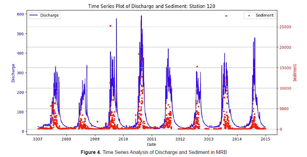
The time series analysis (figure 4) of discharge and sediment concentration at Station 120 in the Mahakali River Basin reveals a strong seasonal pattern, with peak flows and elevated sediment levels occurring annually during the monsoon season. These peaks are driven by intense rainfall and runoff, which enhance erosion and sediment mobilization. Sediment concentration is closely correlated with discharge, indicating that high-flow events dominate sediment transport dynamics. A gradual decline in both variables is observed during the post- monsoon and dry seasons (Figure 4).

Figure 4: Time Series Analysis of Discharge and Sediment in MRB

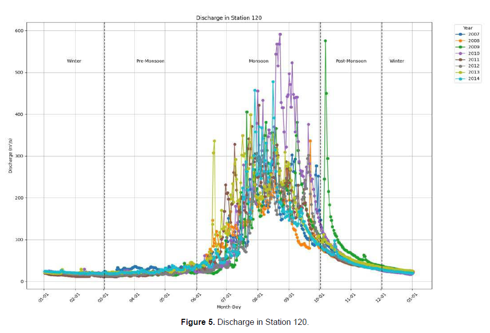
Figure 5 shows the daily discharge at Station 120 from 2007 to 2014, categorized into seasonal periods: Winter, Pre- Monsoon, Monsoon, Post- Monsoon, and Winter. Discharge remains relatively low and stable during the Winter and Pre- Monsoon periods but rises sharply during the Monsoon season, peaking significantly due to heavy rainfall and runoff. After the Monsoon, discharge gradually decreases during the Post-Monsoon period and stabilizes again in Winter.

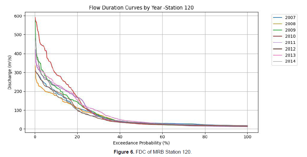
Figure 6 demonstrates flow duration curve for Station 120 from 2007 to 2014. The steep initial slopes of the curves indicate that high discharge events, such as those occurring during the monsoon, are infrequent, while the flatter portions suggest that low to moderate flows occur more consistently throughout the year. Variations between years reflect interannual differences in hydrological conditions, such as rainfall intensity or watershed characteristics.(Figure 5, Figure 6).

Figure 5: Discharge in Station 120.

Figure 6: FDC of MRB Station 120.

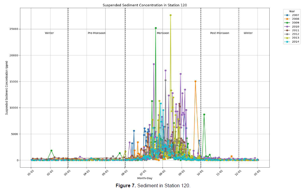
seasonal variation in suspended sediment concentration at Station 120 from 2007 to 2014 with calendar year divided into seasonal periods (Winter, Pre-Monsoon, Monsoon, Post-Monsoon). Data points shows that sediment concentrations are generally low during the Winter and Pre-Monsoon seasons. However, there is a significant spike during the Monsoon season, with peak values exceeding 25,000 ppm in some years, indicating intense sediment transport due to heavy rainfall and runoff. Post-Monsoon sediment levels gradually decrease before stabilizing in Winter. The interannual variability in peak concentrations suggests differences in monsoon intensity or catchment conditions across years (Figure 7).

Figure 7: Sediment in Station 120.

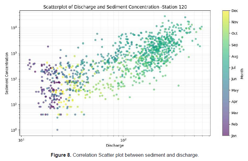
The analysis on sediment discharge relation shows a clear positive correlation at Station 120, with higher sediment concentrations occurring during periods of elevated discharge. This relationship is visually demonstrated in Figure 8, a scatterplot showing the association between discharge and sediment concentration in logarithmic scale. Points corresponding to the monsoon months, represented by green to teal colours, cluster predominantly in the upper- right section of the plot. This clustering indicates that intense sediment transport Occurs during high-flow events driven by heavy rainfall during the monsoon season. In contrast, data points from non- monsoon months, depicted in purple to yellow colors, are concentrated in the lower-left region, reflecting lower discharge and sediment levels during these periods. The seasonal gradient in the scatterplot underscores the strong influence of hydrological patterns on sediment dynamics (Figure 8).

Figure 8: Correlation Scatter plot between sediment and discharge.

Further statistical analysis was performed to confirms this relationship showing moderate positive correlation coefficient (R = 0.6) between discharge and sediment concentration at Station 120 highlights that higher discharge levels are generally associated with increased sediment concentrations. This finding aligns with the expected behaviour of sediment transport, where higher flows enhance erosion and mobilization of sediments, particularly during the monsoon when rainfall intensifies runoff and sediment movement.

Seasonal Variation

Pre- Monsoon Analysis

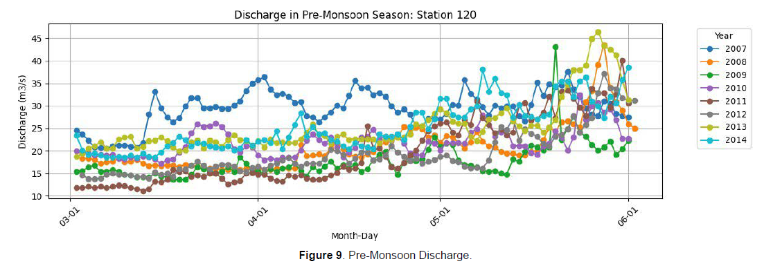
The Pre-Monsoon season (March–May) at Station 120 (Chamelia River) exhibits distinct hydrological and sediment transport dynamics driven by seasonal climatic factors. Figure 9 illustrates the daily discharge patterns during this period, showing a gradual increase in flow from March to late May, ranging between 10 and 45 m³/s. This trend is primarily attributed to snowmelt from higher elevations and occasional pre-monsoon rainfall events. Year-to-year variability is evident, with some years (e.g., 2010 and 2014) experiencing higher peak discharges (~40–45 m³/s), reflecting interannual differences in snowmelt and precipitation. Daily fluctuations are minimal in early March but become more pronounced in late May, indicating periodic runoff events (Figure 9).

Figure 9: Pre-Monsoon Discharge.

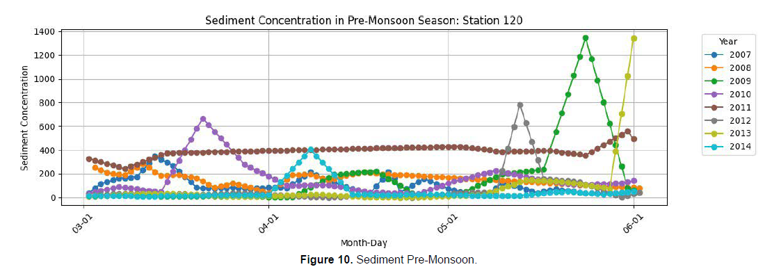
Sediment concentration data during the Pre-Monsoon season, presented in Figure 10, reveal a similar seasonal pattern. Sediment concentrations remain relatively low in March and April, typically below 500 ppm, but show a noticeable increase in May, with sharp spikes near the end of the season. Significant year-to-year variability is observed, with notable peaks in 2010, 2013, and 2014, likely due to localized pre-monsoon rainfall or erosion events. The irregular high sediment concentrations highlight the influence of upstream runoff and erosion processes, which intensify toward the end of the Pre-Monsoon period (Figure 10).

Figure 10: Sediment Pre-Monsoon.

Figure 11 provides insights into the daily average sediment concentration during the Pre-Monsoon season, showing a gradual rise from March (~100 ppm) through April, peaking in late May (~275 ppm). Fluctuations throughout the season reflect the dynamic nature of sediment transport, with increased runoff and erosion contributing to sharper peaks in late April and May. Similarly, Figure 12 depicts the daily average discharge, starting low in early March (~17.5 m³/s) and gradually increasing to ~32.5 m³/s by late May. The consistent upward trend underscores the role of snowmelt and pre-monsoon rainfall in driving discharge increases, with sharper rises in late May signaling intensified runoff. (Figure 11, 12).

Figure 11: Daily Average Pre-Monsoon Sediment.

Figure 12: Pre-Monsoon Daily Average Discharge.

A strong positive correlation (0.75) greater than overall correlation (0.60) between discharge and sediment concentration during the Pre-Monsoon season further emphasizes the close linkage between these variables. This correlation analysis suggests that the rating curve development based upon the season is more reliable than overall rating curve. This relationship highlights that higher discharge levels are generally associated with elevated sediment transport, driven by enhanced erosion and mobilization of sediments during periods of increased runoff. Overall, the Pre-Monsoon season demonstrates a gradual build-up of hydrological activity, setting the stage for the intense sediment transport observed during the subsequent Monsoon period.

Monsoon season

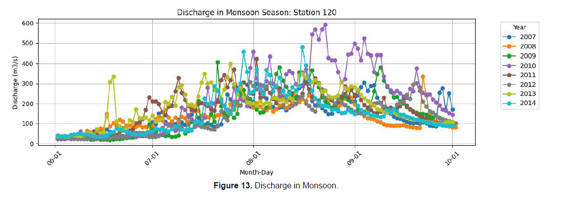
The Monsoon season (June–September) at Station 120 (Chamelia River) is characterized by intense hydrological activity and significant sediment transport, driven primarily by heavy rainfall and runoff. Figure 13 illustrates the daily discharge patterns during this period, showing a sharp rise in flow starting in June, peaking in July and August (~500–600 m³/s in some years), and gradually declining by September. Year-to-year variability is evident, with notable differences in peak discharge. The wide fluctuations in discharge reflect the dynamic nature of monsoon rainfall events, emphasizing the season’s dominant role in driving high discharge variability and peak flows (Figure 13).

Figure 13: Discharge in Monsoon.

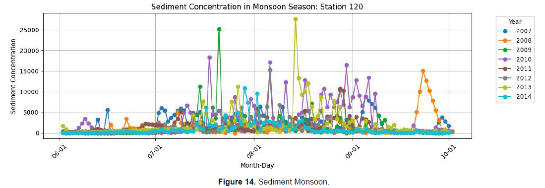
Sediment concentration data during the Monsoon season, presented in Figure 14, reveal an equally pronounced seasonal trend. Sediment concentrations increase significantly throughout the monsoon, with sharp peaks observed across the season. Concentrations vary widely, reaching maximum values exceeding 25,000 ppm in some years. Year-to-year variability in peak sediment concentrations highlights the influence of factors such as rainfall intensity and upstream sediment supply. Notably, late July to early August shows the highest spikes, indicating periods of intense sediment mobilization due to heavy rainfall and erosion (Figure 14).

Figure 14: Sediment Monsoon.

Figure 15 provides insights into the daily average sediment concentration during the Monsoon season, showing a consistent upward trend from early June, peaking in July and August (~5,000 ppm), and gradually declining by late September. Significant daily variability is observed, with sharp spikes reflecting intense sediment transport events. These peaks align closely with the peak monsoon period, driven by heavy rainfall and runoff, underscoring the monsoon’s critical role in sediment mobilization (Figure 15).

Figure 15: Daily Average Sediment Monsoon.

Daily average discharge patterns during the Monsoon season, depicted in Figure 16, further highlight the seasonal dynamics. Discharge rises steadily from early June, reaches its peak in July and August (~300 m³/s), and gradually declines through September. The highest discharge occurs in late July, corresponding to peak monsoon rainfall and runoff. Daily fluctuations are evident, but the overall pattern reflects a consistent seasonal rise and fall, reinforcing the monsoon’s significant impact on river discharge (Figure 16)

Figure 16: Daily Average Discharge Monsoon.

A strong positive correlation coefficient of 0.76 indicates that higher discharge is closely associated with higher sediment concentration. This robust linkage underscores the dominant role of monsoon flows in sediment mobilization, where increased runoff enhances erosion and sediment transport. The perfect correlation along the diagonal confirms the self-consistency of each variable, while the strong off-diagonal relationships emphasize the tight coupling between discharge and sediment dynamics during this period.

Post-Monsoon Season

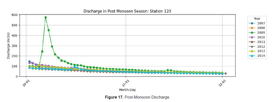
The Post-Monsoon season (October–November) at Station 120 (Chamelia River) marks a transitional phase characterized by a steady decline in hydrological and sediment transport activity following the peak monsoon period. Figure 17 shows that discharge begins high in early October reaching up to ~500 m³/s in 2009 due to residual runoff from the monsoon then declines steadily to base flow levels of approximately 50 m³/s by late November. This consistent downward trend reflects the rapid reduction in rainfall and surface runoff as the monsoon recedes. While year-to-year variability is observed in the initial peak flows, with 2009 showing the highest early-season discharge, the overall pattern across all years indicates a gradual return to stable low-flow conditions (Figure 17).

Figure 17: Post-Monsoon Discharge.

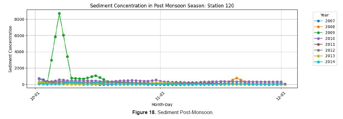
Sediment concentration during this season, as shown in Figure 18, is generally low, with most values remaining below 500 ppm. However, a notable exception occurred in early October 2009, when a sharp spike in sediment concentration (~8,000 ppm) was recorded, likely due to a localized high-intensity rainfall event, delayed erosion

response, or upstream geomorphic disturbance. Most other years exhibit minimal sediment transport, underscoring the season’s typically low sediment load (Figure 18).

Figure 18: Sediment Post-Monsoon.

The daily average sediment concentration (Figure 19) further illustrates this trend, showing a pronounced peak (~1,200 ppm) in early October, followed by a steady decline to 100–200 ppm by November. This early-season spike suggests residual sediment mobilization from the tail end of the monsoon or isolated runoff events, which diminish as catchment stabilization occurs (Figure 19)

Figure 19: Daily Average Post Monsoon Sediment.

Similarly, the daily average discharge (Figure 20) starts at ~140 m³/s in early October and decreases steadily to around 40 m³/s by the end of November, with a sharp initial drop followed by a gradual decline. This pattern confirms the transition from monsoon-influenced high flows to base flow-dominated conditions (Figure 20).

Figure 20: Daily Average Post-Monsoon Discharge.

Despite the overall reduction in flow and sediment, the correlation analysis reveals a strong positive relationship between discharge and sediment concentration during the Post-Monsoon season, with a correlation coefficient of

0.86. This indicates that even during this low-flow period, sediment transport remains closely tied to discharge dynamics, particularly during the early phase when residual runoff continues to influence sediment mobilization.

Winter Season

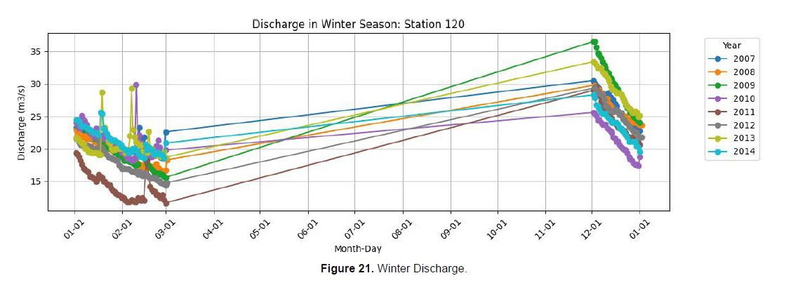
The Winter season (December–February) at Station 120 (Chamelia River) is characterized by stable, low- flow conditions with minimal hydrological and sediment transport activity. Figure 21 shows that daily discharge remains consistently low, ranging between 15–30 m³/s, reflecting sustained baseflow regimes with limited influence from precipitation or snowmelt during this dry period (Figure 21).

Figure 21: Winter Discharge.

The daily average discharge (Figure 22) shows a gradual decline from approximately 22 m³/s in early January to around 18 m³/s by February. Overall, the hydrological system exhibits high stability, typical of winter baseflow conditions in the region (Figure 22).

Figure 22: Daily Average Discharge Winter.

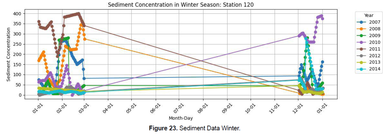
Sediment concentration during winter is generally very low, with most values below 50 ppm (Figure 23). However, occasional spikes-reaching up to 400 ppm in 2010 and 2014—indicate episodic sediment mobilization, potentially due to localized rainfall, slope failures, or human-induced disturbances (Figure 23).

Figure 23: Sediment Data Winter.

The daily average sediment concentration (Figure 24) remains low (~80–100 ppm) throughout the season, with a modest peak of ~180 ppm in early February, suggesting limited but intermittent sediment supply. These fluctuations underscore that while the winter season is largely inactive in terms of erosion and transport, short-lived events can still trigger measurable sediment pulses (Figure 24).

Figure 24: Daily Average Sediment Winter.

A weak negative correlation (−0.45) between average discharge and sediment concentration during winter. This inverse relationship suggests that higher discharge values are slightly associated with lower sediment concentrations, which may seem counterintuitive but can be explained by the dominance of groundwater driven base flow, where increased subsurface flow dilutes sediment concentration. Additionally, limited sediment availability in the channel and catchment during the dry season restricts erosion, even during minor flow increases. The lack of readily erodible material and reduced surface runoff diminish the typical discharge sediment linkage observed in wetter seasons.

Processed Daily Average Data

To ensure data quality and improve the reliability of seasonal sediment-discharge relationships, a filtering process was applied to remove outliers from the daily average sediment and discharge datasets for each of the four hydrological seasons Pre-Monsoon, Monsoon, Post-Monsoon, and Winter. Outliers were identified and removed using the Interquartile Range (IQR) method, where values falling below Q1 − 1.5×IQR or above Q3 + 1.5×IQR were considered outliers. Following Figure 25 to 32 represents the filtered data of daily average discharge and sediment (Figure 25-32).

Figure 25: Pre-Monsoon Filtered Discharge.

Figure 26: Filtered Pre-Monsoon Sediment.

Figure 27: Filtered Monsoon Discharge.

Figure 28: Filtered Monsoon Sediment.

Figure 29: Filtered Post Monsoon Discharge.

Figure 30: Filtered Post Monsoon Sediment.

Figure 31: Filtered Winter Discharge.

Figure 32: Filtered Winter Sediment.

Model Development

Three different model namely KNN, SVM and Random forest has been developed for each season with findings as follows.

KNN Pre-Monsoon

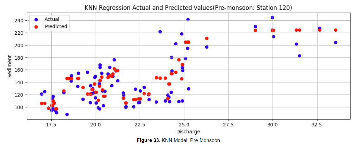
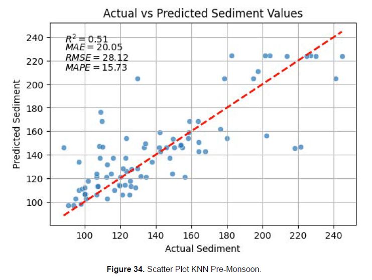
The KNN regression model was developed to predict suspended sediment concentration based on discharge during the Pre- Monsoon season at Station 120 in the Mahakali River Basin. As shown in Figure 33, the predicted sediment values (red points) generally follow the trend of the actual observed values (blue points), Figure 33 KNN Model, Pre-Monsoon indicating that the model captures the overall relationship between discharge and sediment transport. Performance is relatively better at lower discharge ranges (~17.5–22.5 m³/s), where predictions align closely with observations, but increases in variability are evident at higher discharges (~25–32.5 m³/s), with instances of both under- and over-prediction. This suggests that KNN, while effective in capturing local patterns, may struggle with extrapolation or generalization in data-sparse or high-variability regions. The scatter plot in Figure 34 further illustrates this behavior, where most data points cluster near the 1:1 line at lower sediment concentrations, but significant scatter occurs at higher values. Model evaluation metrics R² = 0.51, MAE = 20.05 ppm, RMSE = 28.12 ppm, and MAPE = 15.73% indicate moderate predictive accuracy, with the model explaining just over half of the variance in sediment concentration. The relatively high RMSE compared to MAE suggests that larger errors disproportionately influence model performance, particularly during high-sediment events (Figure 34)

Figure 33: KNN Model, Pre-Monsoon.

Figure 34: Scatter Plot KNN Pre-Monsoon.

KNN Monsoon

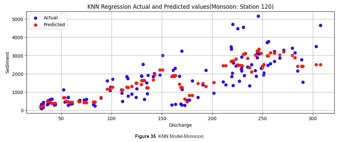
The KNN regression model was evaluated for its ability to predict suspended sediment concentration during the Monsoon season at Station 120 in the Mahakali River Basin. As illustrated in Figure 35, the predicted sediment values generally follow the trend of the observed data, particularly at low discharge levels (~0–100 m³/s), where predictions align reasonably well despite some underestimation. However, as discharge increases, the model's performance deteriorates. In the mid-range (100–250 m³/s), predictions become more scattered, indicating inconsistent accuracy, while at high discharges (~250–300 m³/s), the model significantly underestimates sediment concentrations—critical during peak monsoon events when sediment loads are highest. This suggests that KNN struggles to capture the nonlinear and highly variable sediment dynamics under extreme flow conditions, likely due to sparse data coverage and its sensitivity to local neighbourhood patterns (Figure 35).

Figure 35: KNN Model-Monsoon.

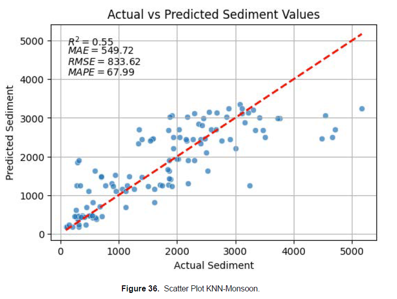
The scatter plot in Figure 36 further confirms these limitations, showing good agreement between actual and predicted values at lower sediment levels (<1000 ppm), with points clustering near the 1:1 line. However, for higher sediment concentrations (>2000 ppm), there is substantial scatter and a clear tendency for underprediction. Model performance metrics R² = 0.55, MAE = 549.72 ppm, RMSE = 833.62 ppm, and MAPE = 67.99% reflect moderate explanatory power but highlight significant prediction errors, particularly in magnitude. The high RMSE and MAPE values indicate that large deviations, especially during high-flow events, disproportionately affect model accuracy. While the KNN model captures general trends in sediment transport during the monsoon, its inability to accurately predict peak sediment loads limits its reliability for applications requiring precise estimation under extreme conditions. These findings underscore the need for more robust modeling techniques capable of handling the high variability and nonlinearity inherent in monsoon- driven sediment transport systems.

KNN Post Monsoon

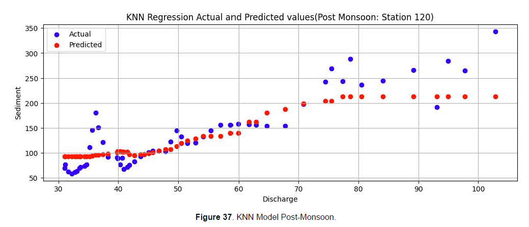
The KNN regression model demonstrates moderate performance in predicting suspended sediment concentrations during the Post- Monsoon season at Station 120 in the Mahakali River Basin. As shown in Figure 37, the predicted values (red points) generally follow the trend of the observed data, particularly at lower discharge range, where predictions align closely with actual sediment levels. However, deviations become more apparent in the mid-range (~50–70 m³/s), with a tendency for underestimation, and are most pronounced at higher discharges (~70– 100 m³/s), where the model fails to capture the full variability of sediment transport, resulting in significant under predictions. This suggests that while KNN performs well in stable, low-flow conditions, it struggles to adapt to dynamic or high-magnitude events where data sparsity and nonlinear responses limit its predictive accuracy.

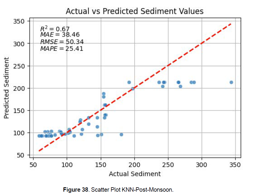
The scatter plot in Figure 38 further illustrates model performance, with most points clustering near the 1:1 line for lower sediment concentrations (<150 ppm), indicating reliable predictions in this range. For higher sediment levels (>200 ppm), increased scatter and systematic underestimation are evident. Performance metrics R² = 0.67, MAE = 38.46 ppm, RMSE = 50.34 ppm, and MAPE = 25.41% confirm moderate predictive capability, with the model explaining a substantial portion of the variance in sediment concentration. The relatively low MAE suggests good average performance, but the growing divergence at higher values highlights limitations in capturing extreme events (Figure 36-38).

Figure 36: Scatter Plot KNN-Monsoon.

Figure 37: KNN Model Post-Monsoon.

Figure 38: Scatter Plot KNN-Post-Monsoon.

KNN Winter

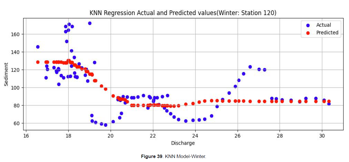
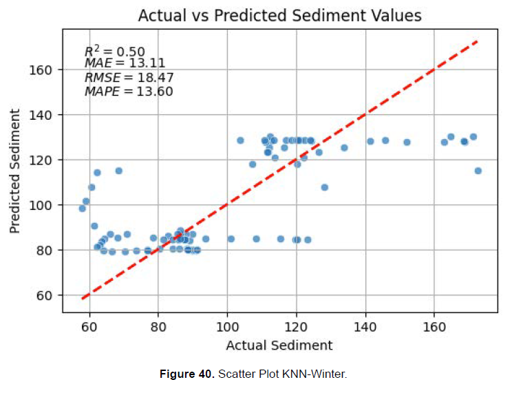
The KNN regression model exhibits moderate performance in predicting suspended sediment concentrations during the Winter season at Station 120 in the Mahakali River Basin, but struggles to capture the observed variability despite while the predicted values follow a relatively consistent trend, they fail to reflect the actual fluctuations in sediment concentration across all discharge ranges. At low discharges (~16–18 m³/s), the model underestimates peak sediment values, where observed levels vary widely (80–160 ppm), while predictions remain clustered around 80–90 ppm. In the mid-range (~20–24 m³/s), actual sediment values show continued variability, but the model output remains flat, indicating poor sensitivity to changes in transport dynamics. At higher discharges (~26– 30 m³/s), where a slight increasing trend is evident in the actual data, the model fails to respond, resulting in persistent underestimation. This suggests that KNN has limited (Figure 39, 40).

Figure 39: KNN Model-Winter.

Figure 40: Scatter Plot KNN-Winter.

Capacity to capture non-linear or episodic sediment responses during winter, possibly due to sparse data or the dominance of isolated events not well-represented in the training set. The scatter plot in Figure 39 further confirms these limitations, with most points clustered near the 1:1 line for lower sediment concentrations (~60–120 ppm), indicating acceptable performance in the average range. However, significant scatter and under prediction occur at higher sediment levels (>120 ppm). Model evaluation Metrics-R² = 0.50, MAE = 13.11 ppm, RMSE = 18.47 ppm, and MAPE = 13.60%-reflect moderate accuracy, with half of the variance in sediment concentration unexplained. The low MAE suggests reasonable average performance, but the R² and visible underestimation of peaks indicate poor explanatory power for extreme values.

SVM Model Pre-Monsoon

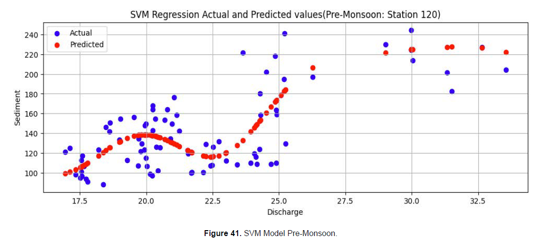
The Support Vector Machine (SVM) regression model demonstrates improved performance in predicting suspended sediment concentrations during the Pre-Monsoon season at Station 120 in the Mahakali River Basin. As shown in Figure 41, the predicted values generally follow the trend of the observed sediment data fluctuations. However, as discharge increases beyond ~24 m³/s, the predicted values align closely with the observed trend, demonstrating the model’s ability to capture the rising sediment transport more accurately. The smoothing nature of SVM helps in approximating the overall pattern, though it tends to average out some of the finer- scale variations.

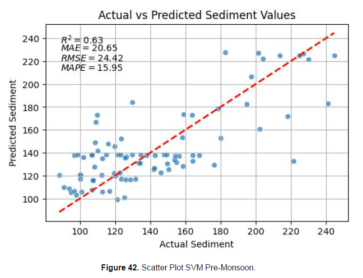
This performance is further validated in Figure 42, which plots actual versus predicted sediment concentrations. The data points show reasonable agreement along the 1:1 line, particularly in the mid to higher sediment range. Model evaluation metrics R² = 0.63, MAE = 20.65 ppm, RMSE = 24.42 ppm, and MAPE = 15.95% indicate moderate to good predictive accuracy. The R² value suggests that 63% of the variance in sediment concentration is explained by the model, while the relatively low MAE and MAPE reflect acceptable average error levels. These results highlight SVM’s strength in capturing the overall sediment-discharge relationship, particularly during periods of increasing flow, and its robustness in handling moderate non-linearity (Figure 41, 42).

Figure 41: SVM Model Pre-Monsoon.

Figure 42: Scatter Plot SVM Pre-Monsoon.

SVM Monsoon

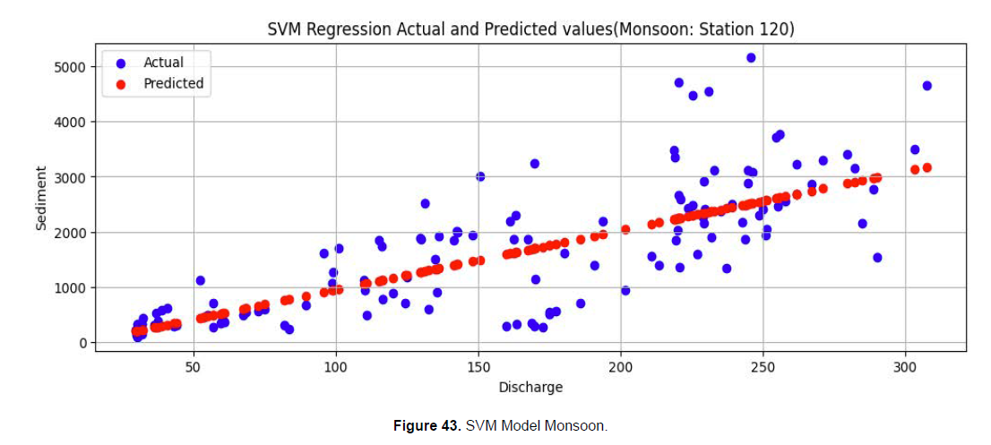
(Figure 43) and extreme sediment variability. As shown in Figure 43, the actual sediment values exhibit a generally increasing trend with discharge (~30–300 m³/s), but with significant scatter—particularly at higher flows—reflecting the complex and dynamic nature of sediment transport during intense rainfall events. The predicted values follow a smoother, more linear trend, indicating that the SVM model captures the overall relationship between discharge and sediment, but fails to reproduce the finer-scale fluctuations and peak events. At lower discharges (30–100 m³/s), the model aligns reasonably well with observed values. However, in the mid-range (150–250 m³/s), it smooths out variability, and at higher discharges (>250 m³/s), it consistently underestimates peak sediment concentrations, which are critical for accurate sediment load estimation (Figure 44)

Figure 43: SVM Model Monsoon.

Figure 44: Scatter Plot SVM-Monsoon.

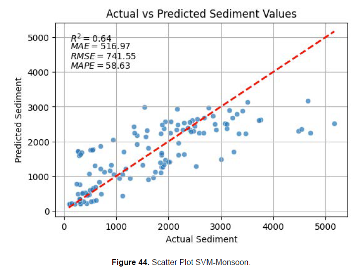
This limitation is further confirmed in Figure 44, which plots actual versus predicted sediment values. While data points are moderately clustered around the 1:1 line at lower sediment levels, there is substantial scatter at higher concentrations (>2000 ppm), with most predictions falling below the ideal line. Performance metrics R² = 0.64, MAE = 516.97 ppm, RMSE = 741.55 ppm, and MAPE = 58.63% indicate moderate explanatory power but highlight significant predictive errors. Although the model explains 64% of the variance in sediment data, the high MAPE and RMSE values reflect large relative and absolute deviations, particularly during extreme events. The smoothing behaviour of SVM, while beneficial in reducing noise, limits its ability to capture non-linear spikes and hysteresis effects prevalent in monsoon-driven systems.

SVM Post-Monsoon

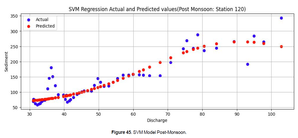
The Support Vector Machine (SVM) regression model demonstrates strong performance in predicting suspended sediment concentrations during the Post-Monsoon season at Station 120 in the Mahakali River Basin. As shown in Figure 45, the actual sediment values exhibit a generally increasing but non-linear relationship with discharge (~30–105 m³/s), reflecting residual monsoon effects and variable sediment availability. The predicted values follow a smoother trend that captures the overall pattern, though some finer-scale fluctuations and peak events are not fully reproduced, particularly at higher discharges. At lower flows (30–40 m³/s), discharges (>70 m³/s), the model tends to underestimate peak sediment concentrations, revealing limitations in capturing extreme events due to data sparsity and the inherent smoothing behaviour of SVM (Figure 45).

Figure 45: SVM Model Post-Monsoon.

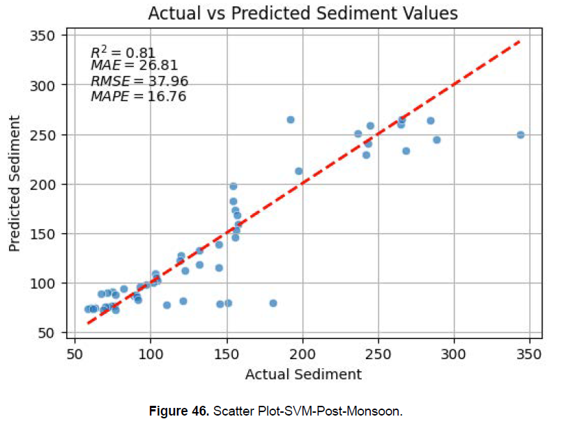
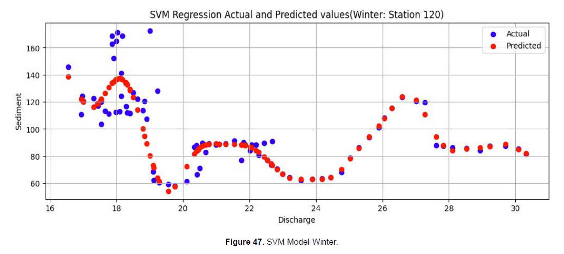
This performance is further validated in Figure 46, where actual versus predicted sediment values show tight clustering around the 1:1 line, especially for concentrations below 150 ppm. The model achieves a high coefficient of determination (R² = 0.81), indicating that it explains 81% of the variance in sediment data among the best seasonal performances observed. The MAE of 26.81 ppm and RMSE of 37.96 ppm reflect low to moderate absolute errors, while the MAPE of 16.76% suggests acceptable relative accuracy across most of the range. These metrics confirm that SVM performs reliably during the Post-Pulses. As illustrated in Figure 47, the actual sediment values exhibit a complex, non-linear relationship with discharge (~16–30 m³/s), including an initial peak, a sharp decline, and a subsequent rise at higher discharges. These fluctuations likely reflect isolated runoff events, groundwater seepage, or localized erosion rather than consistent hydrological drivers (Figure 46).

Figure 46: Scatter Plot-SVM-Post-Monsoon.

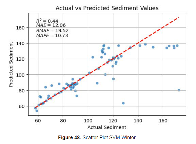
The predicted values capture broad trends such as the initial peak and later increase but fail to reproduce abrupt changes, instead smoothing out critical variations due to SVM’s inherent regularization and tendency to prioritize generalization over local detail (Figure 47, 48).

Figure 47: SVM Model-Winter.

Figure 48: Scatter Plot SVM-Winter.

This limitation is evident in the actual vs. predicted scatter plot (Figure 48), where data points show considerable scatter around the 1:1 line, indicating a weak fit. The model achieves an R² of only 0.44, meaning it explains less than half of the variance in observed sediment concentrations—among the lowest performances across all seasons. While the MAE (12.06 ppm) and RMSE (19.52 ppm) suggest relatively small average errors, the MAPE of 10.73% must be interpreted cautiously given the low absolute sediment range; the model performs reasonably well on average but fails to capture high-magnitude deviations. The poor R² and visual scatter confirm that SVM struggles to represent the non-linear and sporadic nature of winter sediment dynamics, particularly during sudden sediment pulses not well-correlated with discharge.

Random Forest Pre-Monsoon

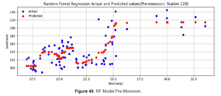
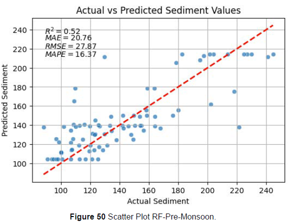
and somewhat variable relationship with discharge (~17– 33 m³/s), reflecting the influence of snowmelt and sporadic pre- monsoon rainfall. The predicted values follow the general trend, particularly at higher discharges (25–33 m³/s), where the model captures the increasing sediment transport with notable accuracy. However, in the lower to mid- discharge range (18–24 m³/s), predictions display significant smoothing, failing to reproduce local peaks and fluctuations, which indicates the model’s tendency to average out fine-scale variability despite its ensemble nature. This behaviour is further reflected in Figure 50, which plots actual versus predicted sediment values. While most data points cluster around the 1:1 line, suggesting reasonable agreement, there is visible scatter and systematic under- or over-prediction at certain levels. Performance Metrics-R² = 0.52, MAE = 20.76 ppm, RMSE = 27.87 ppm, and MAPE = 16.37%-confirm moderate predictive accuracy. The model explains just over half of the variance in sediment concentration, with acceptable average error levels, indicating its capability to capture general trends but limited skill in reproducing high-frequency variations (Figure 49, 50).

Figure 49: RF Model Pre-Monsoon.

Figure 50: Scatter Plot RF-Pre-Monsoon.

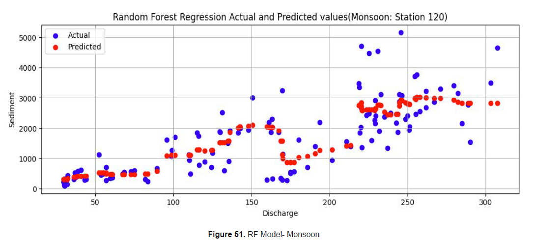
loads. As shown in Figure 51, the predicted values generally follow the overall increasing trend of the actual sediment data across the discharge range of ~30–300 m³/s. However, significant deviations are evident, particularly at higher discharges (180–300 m³/s), where the model fails to capture peak sediment events and instead produces smoothed predictions that underestimate the most intense sediment pulses. This smoothing effect reflects RF’s ensemble averaging mechanism, which enhances stability but reduces sensitivity to extreme or rare events (Figure 51, 52).

Figure 51: RF Model- Monsoon

Figure 52: Scatter Plot RF-Monsoon.

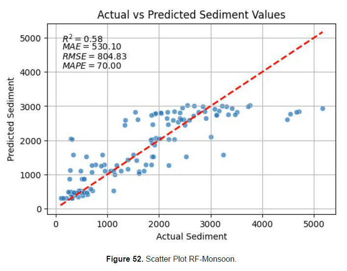
The scatter plot in Figure 52

Figure 51 Random Forest Model Monsoon

Figure 52 Scatter Plot RF Monsoon

Further illustrates this limitation, showing that while data points are reasonably clustered at lower sediment concentrations (<1000 ppm), there is substantial scatter at higher values, with most predictions falling below the 1:1 line. This indicates systematic underestimation of extreme sediment transport events, which are critical for accurate sediment budgeting and infrastructure planning. Model performance metrics R² = 0.58, MAE = 530.10 ppm, RMSE = 804.83 ppm, and MAPE = 70.00% confirm only moderate explanatory power and high prediction error. While the model explains 58% of the variance in sediment data, the MAE and RMSE values are relatively large, and the exceptionally high MAPE reveals that, on average, predictions deviate from observations by 70%, rendering the model unreliable for precise estimation during peak monsoon conditions. (Figure 53).

Figure 53: RF Model-Post-Monsoon.

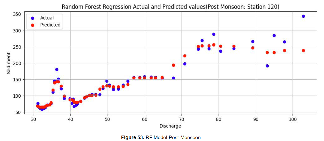
The Post-Monsoon season at Station 120 in the Mahakali River Basin. As shown in Figure 53, the predicted values closely follow the trend of the actual sediment data across the discharge range of ~30–105 m³/s. The model captures the increasing sediment trend with high fidelity, particularly at lower to moderate sediment levels (below ~200 ppm), where predictions align tightly with observations. Even in regions of moderate variability, such as discharge between 30–45 m³/s, the model exhibits strong tracking, indicating its ability to reproduce observed patterns with minimal deviation (Figure 54).

Figure 54: Scatter Plot-RF-Post-Monsoon.

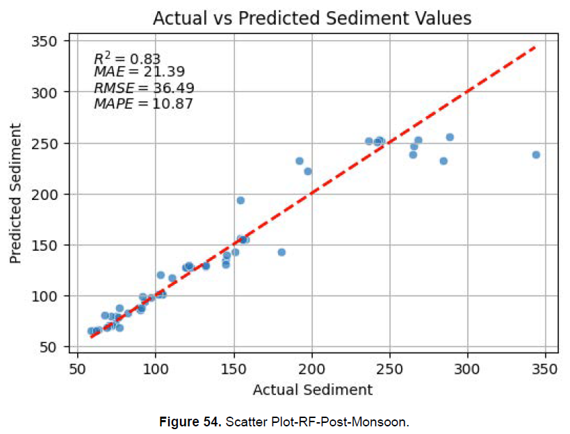
This high level of accuracy is further confirmed in Figure 54, where actual versus predicted sediment values show tight clustering around the 1:1 line, reflecting a robust model fit. The performance metrics R² = 0.83, MAE = 21.39 ppm, RMSE = 36.49 ppm, and MAPE = 10.87% underscore the model’s superior predictive capability. The high R² value indicates that 83% of the variance in sediment concentration is explained by the model, while the low MAE and MAPE values reflect minimal average error and high relative accuracy.

Random Forest Winter The Random Forest (RF) regression model shows limited predictive skill in estimating suspended sediment concentrations during the Winter season at Station 120 in the Mahakali River Basin, despite low and stable hydrological conditions. As illustrated in (Figure 55), the actual sediment values exhibit high variability across a narrow discharge range (~16–30 m³/s), with distinct peaks around 18 and 26 m³/s, likely reflecting isolated sediment mobilization events such as localized runoff, slope failures, or groundwater seepage. While the predicted values (red dots) align reasonably well in certain segments particularly between discharges of ~20 - 25 m³/s and above ~27 m³/s the model fails to capture the full range of observed fluctuations, especially sharp sediment spikes, indicating a lack of sensitivity to episodic dynamics.