Sensitivity Analysis of CALPUFF Model: Application Over Complex Terrain
Received: 10-Apr-2021 / Accepted Date: 21-Apr-2021 / Published Date: 29-Apr-2021 DOI: 10.4172/2157-7617.1000559
Abstract
Parameterization study of CALMET/CALPUFF modeling system was performed in a short term short range release scenario over complex terrain in Pakistan. A comprehensive dataset developed through a tracer field experiment was used to analyze its performance in a mountainous region in Islamabad city. In most complex terrain regions of world and especially in Pakistan, scarcely located observational stations cannot provide spatial variability of meteorological fields, especially the turbulent parameters over complex terrain. Therefore, use of prognostic model seems to be imperative for adequate meteorological input to dispersion model. For this purpose meso-scale meteorological model WRF was coupled with CALPUFF to provide 3D meteorological input. Parameterization study of CALMET and CALPUFF was performed to find out the best configuration of model for current meteorological and topographical conditions of test site. In this regard different computational variants in CALMET/CALPUFF were tested and their impact on pollutant concentration was analyzed using standard statistical indices. The best results were achieved for the CALMET grid resolution of 300 m, SRTM3 dataset and high temporal resolution of meteorological input into CALPUFF. The selection of appropriate dispersion coefficients is imperative for simulations over complex terrain. Dispersion coefficients based on similarity theory provided better results as compared to dispersion coefficients derived from Pasquill-Gifford (PG) curves in short term release scenarios. Model strongly under-predicts at lower concentration at receptors away from source and starts to perform better at higher concentrations. However, peak concentration was slightly underestimated in this experiment. CALPUFF model has proven to fulfill criteria for a ‘good’ dispersion model for application over complex terrain for short term short range release scenarios, when used with prognostic meteorological data option only.
Keywords: CALPUFF model; Complex terrain
Introduction
CALPUFF modeling system is an alternative to recommended models by US EPA for regulatory purposes. It can be used for studying atmospheric dispersion in long range and on a case by case basis short range with non-homogeneous meteorological conditions. CALPUFF is a more accurate and representative model than ISCST3, AERMOD or CTDM especially in its treatment of meteorology and complex terrain. CTSG (Complex Terrain Algorithm for Subgrid Features) concept is utilized by CALPUFF to compute puff trajectories in complex terrain [1]. Meteorological data is a key input that is provided to run atmospheric dispersion modeling system. CALMET/CALPUFF modeling system [2] has capability to simulate pollutant transport and dispersion within non-homogeneous meteorological fields, though application of these models greatly depends upon the availability of meteorological data sets that can precisely resolve Planetary Boundary Layer (PBL) structure. Observational data, in most cases, are limited and cannot adequately resolve details of the meteorological fields. Dynamical models have the capability to realistically simulate mesoscale meteorological fields which cannot be totally resolved by sparsely available observations only. A number of studies have been conducted to assess the coupling of WRF with the CALMET model. The meso-scale model WRF was coupled with the diagnostic model CALMET (WRF/ CALMET system) over a complex terrain and coastal domain in NW of Spain. For validation, primary pollutants ground level concentration was measured. The best surface results were obtained by coupling CALMET with WRF to produce meteorological input for dispersion calculations [3]. WRF/CALPUFF coupled modeling system was used to calculate concentration distributions of typical air pollutants (PM10 and SO2) from industrial complexesin Ulsan, Korea. Statistical analysis has also been performed to determine the model’s capability to predict observations [4]. Simulated data was more useful for understanding the pollutant concentration than observational data because measuring sites were sparsely available in the target area. Meteorological fields and dispersion of the pollutants (sulphur and nitrogen dioxides) obtained from coupling of WRF and CALMET modeling systems were compared with the CALMET/CALPUFF model in southeast region of Brazil [5]. In this study, it was concluded that wind direction and dispersion simulation can be considered more realistic using coupled WRF and CALMET modeling system. In previous studies parameterization of CALMET/CALPUFF modeling system were performed using datasets collected from routine release of industrial complexes. The impact of increasing grid resolution on the calculation of maximum concentration field of NOx was studied. Increasing the grid resolution from 1000m to 100m, direct impact on peak concentration value was investigated. For regulatory purposes, the peak concentration should never be underestimated by dispersion model. Highest peak concentration values were obtained using 100m grid resolution, however little discrepancies were found with 250m grid resolution which shortened the run time [6]. Application of CALPUFF model for short term release scenarios in complex terrain has been investigated for different regions. A tracer field experiment was conducted on the bank of Gan Jiang, China to evaluate the real time application of CALPUFF for short term short range dispersion modeling [7]. Results from this experiment showed that CALPUFF model has simulated accurately the direction and position of tracer cloud but under-estimated ground level concentrations and especially peak concentration, which becomes important for regulatory compliance. Authors found that there are some uncertainties in model capability to simulate short-term short-range release scenarios. The model performs better for short as well as long range but for long time average dispersion modeling. The CALPUFF model under-estimate the high ground level concentrations field near to the source. Such scenarios are common in short term release and weak dynamics in complex terrain. In most of these studies, models were tested for regulatory compliance through comparison of high-end simulated and observed concentrations of pollutants. Such evaluation is insufficient as dispersion models can be used to get many goals. The model needs to be tested through comprehensive database developed through field tracer tests over complex terrain for operational purposes by comparing the point to point concentration and evaluating performance variation with increasing distance from source. The optimization of meteorological and dispersion models for short range and short term emergency releases scenarios needs to be evaluated. In present study, coupled meteorological and dispersion modeling system was analyzed using different options like ‘horizontal grid resolution’, ‘temporal resolution of input met data’, ‘dispersion coefficient’ and ‘land used databases’. Aim of this study is parameterization of CALMET/CALPUFF modeling system in short term release scenarios over complex terrain where no observational data from meteorological station is available. Such emergency/routine release scenarios are expected from power plants and other industrial complexes located in mountainous regions. In order to accomplish stated goal, a short term tracer field experiment was performed in the mountainous area of Pakistan. Such studies are important for model configuration and optimization in real time meteorological and topographical conditions of Pakistan, characterized by large topographic diversity and weather variations over short distances.
Methodology
Site description
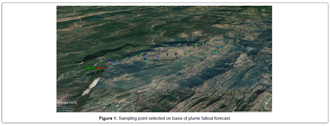
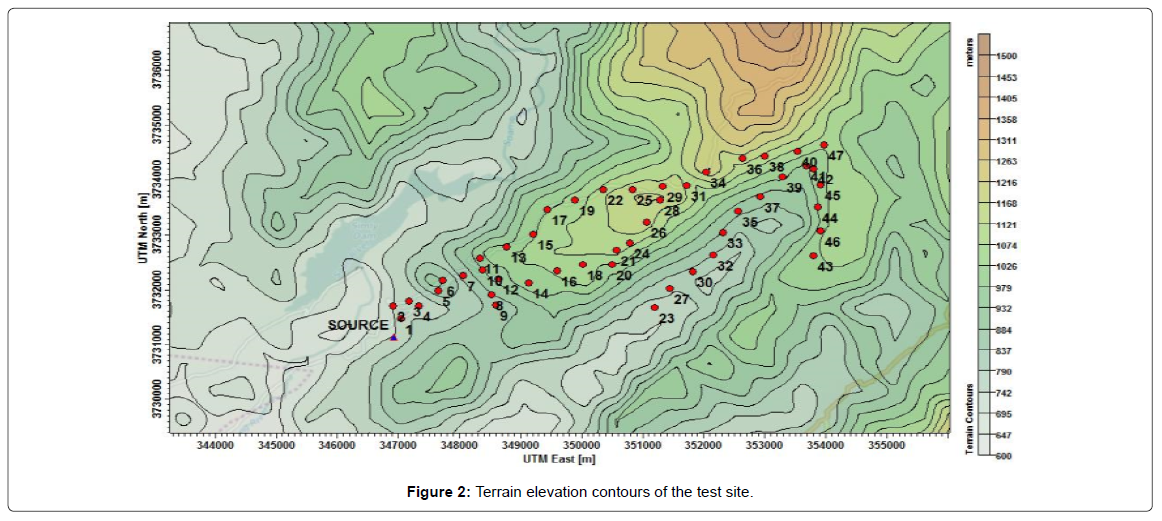
Site for tracer field experiment was selected in hilly mountainous region East of Islamabad. Geographical coordinates of the release point are 33.72⁰ N, 73.38⁰ E. Study domain consists mostly of forest land and mountainous area (Figure 1) gives an overview about geographical environment of the site and receptors position during the tracer field experiment. The highest sampling point is located at 1199 m above mean sea level (Figure 2).
Forecasting of wind field at test site
Accurate forecasting of wind field during tracer test is crucial to select the sampling points, deciding emission time and sampling duration. Wind field study of test site was performed before Page 2 of 8 conducting experiments to simulate synoptic scale wind and local wind circulations due to complex terrain. A single ground weather station will not be sufficient to provide this information due to heterogeneous meteorological conditions of study site. Therefore, WRF model was configured at high resolution of 1 km to simulate meteorological parameters atsite. Wind field forecasting was accomplished usingNCEP GFS data with spatial and temporal resolution of 0.25 degrees and 1 hour respectively. Data for WRF model initialization was downloaded from NCEP/ NOAA website https://ftp.ncep.noaa.gov/data/nccf/com/ gfs/prod/. Diurnal variations of local scale wind circulations at test site were extensively studied. Diagnostic model CALMET was used to further increase horizontal grid resolution up to 300 m. Forecasted meteorological fields were used by dispersion model to predict plume trajectory. Sampling points were decided on the basis of predicted wind speed, wind direction and resultant expected plume fallout.
Field tracer experiment
A field tracer experiment was performed on mountainous complex terrain near Islamabad region on April 21, 2018. Due to hilly area, all locations were not accessible. Therefore, possible routes for deployment and collection ofsamples were selected. A total of 47 discrete sampling points were selected on the basis of wind flow direction and plume fallout forecasted using WRF/CALPUFF. On the basis of average wind direction forecast, receptor positions in the North-East direction of the release point were selected, as shown in Figure 1. Tracer gas (SF6) was released continuously at an average rate of 8 g/s for two hours from a point elevated source. The height of release was 21 m above ground. Release started at 0700 UTC and ended at 0900 UTC. Sampling was started after one hour of release so that sufficient concentration field was developed in sampling region. Nearest sampling point was at 350 m, whereas the farthest point was at 7870 m downwind from release point. Three samples were collected using air samplers at each sampling point in order to calculate hourly average concentration. One sample bag (each with 2 liter capacity) was sampled for 10 min and the interval between two samplings was 10 minutes.
Collected air sample analysis technique
A highly sensitive technique is required to measure the SF6 concentration at ppt level. For this purpose gas chromatography technique with electron capture detector (GC-ECD) was used (detectability limit 5pptv). It is a highly useful technique for analysis of chemical compounds with high electron affinity. The high molecular electro negativity of fluorine in SF6 allows quantification and detection sensitivity at trace level [8]. Samples were analyzed at the gas chromatography laboratory of PIEAS using Gas Chromatograph Thermo Scientific TRACE 1300 Series. Different environmental and system parameters were selected to get stability. Operating parameters for GC-ECD are given in (Table 1). Separation of SF6 was done using packed column of Molecular sieve 5A. For introducing a carrier gas (N2) from cylinder into the GC system, a mass flow controller was used in order to maintain the gas rate at constant flow (30 ml/min). Injection system consisted of an Agilent gas tight syringe of capacity 1 ml. The SF6 gas was injected through septum with injection size of 0.2 ml. Column was baked at 250 °C during measurements to clean out potential contaminants, which may reduce the detector response and peak separating power in long-term. A calibration method for GC-ECD to measure atmospheric concentration of SF6 was developed. GC-ECD was calibrated at the beginning of each analysis day using the laboratory prepared standards. Laboratory standards were stored in evacuated vials. All calibration standards were prepared by mixing calculated amount of SF6 in air. SF6 secondary standard in base gas N2 of 1 ppm (St. dev. = 0.02 ppm) was used to prepare ppt level laboratory standard (100ppt-700ppt), through serial dilution process following the method used by Lim et al. and Jong et al. [9]. A correlation coefficient (R2) of 0.997 was obtained which indicated good correspondence between SF6 concentration and GC-ECD response.
| Operating parameters | Value |
|---|---|
| Column type | Molecular Sieve 5A, I.D. = 2 mm, mesh size = 30/60, length = 2 m |
| Carrier Gas flow rate | N2 at 30 ml/min |
| Injector temperature | Ambient temperature (25 °C) |
| Detector temperature | 150 °C |
| Column temperature | 80 °C (Isothermal) |
Table 1: Operating conditions for GC-ECD.
Configuration of WRF
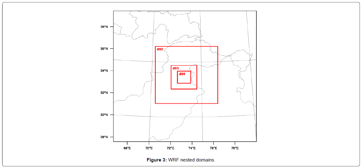
Meso-scale meteorological model WRF [10] (version 3.9) was coupled with diagnostic model CALMET (version 5) to develop meteorological field for CALPUFF (version 7) over study domain. Therefore WRF was configured with high resolution to resolve small scale meteorological features. Four nested domains d01, d02, d03, d04 (Figure 3) of resolution 27 km, 9 km, 3 km and 1 km respectively and 35 vertical sigma levels were defined. Domains d01, d02, d03, d04 had (49×49), (61×61), (76×76) and (121×121) grid cells respectively. Model initial and boundary conditions were provided from 6 hourly (1°×1°) resolution National Center for Environmental Prediction (NCEP) FNL dataset (NCEP). Input parametersfor WRF model are given in (Table 2).
| Name | Description |
|---|---|
| Dynamics | non hydrostatic |
| Horizontal resolution | d01: 27 km, d02: 9 km, d03: 3 km, d04: 1 km |
| Map projection | Mercator |
| Vertical levels | 35 eta levels. |
| Cumulus option | Kain-Fritsch (new Eta) scheme for D01and D02 only. |
| Radiation | RRTM scheme for longwave radiation Dudhia scheme for shortwave radiation |
| Land-surface process | Noah Land-Surface Model (no. of soil layers=4) |
| Surface layer scheme | SL= MM5 Similarity |
| Microphysics | WRF Single-Moment (WSM) 3-class simple ice scheme |
| Boundary layer | ACM2 |
Table 2: Configuration of WRF model.
Configuration of CALMET
Prognostic data option was selected to provide surface and overwater, upper air and precipitation data from WRF. Center of domain was set at release point. CALMET model domain was taken as (20 km × 20 km) with grid spacing of 300 m and 11 vertical layers with cell heights (meters) at 0, 20, 40, 80, 160, 320, 640, 1200, 2000, 3000 and 4000. Shuttle Radar Topography Mission version 2 (SRTM3) has global coverage of terrain elevation at 90 m resolution and was used as input to CALMET. Global Land Cover Characterization (GLCC) is a series of global land cover classification dataset (1-km) and was used as input for land use/land cover (LULC) in CALMET. The specified terrain and land use data files cover the entire meteorological grid.
Computational grid setting and terrain land use/land cover dataset
Grid resolution should be fine enough to resolve small scale terrain features which impact wind flow pattern and aslarge as possible to have small run time and file sizes. Best grid size for a particular application will depend on the size of study domain and complexity of terrain. In order to select an optimum grid size for CALMET/CALPUFF modeling system, grid resolution was varied from 100 m to 1000 m. Upper limit of grid resolution was selected keeping in mind the input meteorological fields from WRF. Adequate grid spacing for a particular application can be selected by comparing the resulting wind field using selected grid spacing with a simulation using twice the resolution (half the grid spacing). If the wind field pattern remains unchanged then the selected grid spacing is suitable. In the present study, optimum grid resolution for the current topographical conditions was determined by calculating its direct impact of concentrations calculation. The Shuttle Radar Topography Mission version 2 (SRTM3) dataset [11], having global coverage of terrain elevation at 90 m resolution, SRTM1 (30 m resolution) and GTOPO (900 m resolution) was used as input into the CALMET. Global Land Cover Characterization (GLCC) (USGS 2010) which is a series of global land cover classification dataset (1-km) was used as input for land use/land cover (LULC) in CALMET. These high resolution spatial datasets enabled CALMET to be configured at fine resolution of 100 m. A number of numerical experiments were performed to find out optimum model configuration using different options for input static datasets and varying grid resolution.
Sub hourly meteorological data as input in the CALPUFF
Steady state Gaussian regulatory models are usually limited to one hour time step and accept only hourly meteorological data input. The CALMET/CALPUFF is the only puff model that can use the subhourly meteorological data [12]. CALMET can correctly predict the flow and direction of wind field, but one hour temporal resolution of meteorological data may be too coarse to predict the short-term dispersion scenario and may induce some errors. The one hour temporal resolution in not sufficient to resolve the subtle fluctuations and variations in the wind field that typically occur in complex terrain under short term release scenarios. The WRF model simulated Meteorological fields have temporal resolution of 1 hour. Therefore, meteorological data input of high temporal resolution of 5 minutes was provided to CALMET to simulate small variations in wind field during experiment. The predicted wind field was greatly improved by increasing the temporal resolution to 5 minutes. The impact of increasing temporal resolution on concentrations was indicated by plotting contours of the spatial distribution of concentrations (section 2.1.3).
Configuration of CALPUFF model
The CALPUFF model was used in default regulatory mode for calculation of concentration of SF6 gas. Chemical transformation, dry and wet deposition was not taken into account because the SF6 was assumed to be chemically inert. The meteorological data fields produced by the CALMET model were used as input to the CALPUFF model. The model default value of 0.5 m/s was used for calm conditions. The value of TERRAD was selected to be 1 km based on the topography of the modeled region. The source parameters were selected the same as in the real-time experiment as given in (Table 3). CALPUFF model provides several different options to select dispersion coefficients which involve input data from three different levels: Dispersion coefficients σ_v and σ_w are computed directly from meteorological tower observation of turbulence. Dispersion coefficients are calculated from micrometeorological variables from CALMET like u^*,w^*, L, h etc., based on similarity theory. Dispersion coefficients extracted from Pasquill-Guifford (PG) stability curves. The default option for dispersion coefficient in CALPUFF is (2), i.e. dispersion coefficients derived from variables calculated from CALMET. The dispersion coefficients based on PG stability curves are normally used in Gaussian plume models [13].
| Parameter | Value |
|---|---|
| Exit temperature | 298 k |
| Exit velocity | 5 m/s |
| Stack diameter | 0.01 m |
| Source elevation | 21 m above ground level/ 751 m a.s.l |
| Source type | Point, elevated, non-buoyant |
| Average wind speed (0700-0900UTC) | 2.48 m/s |
| Average wind direction(0700-0900UTC) | 255 degrees |
Table 3: Summarized source parameters.
Statistical analysis for model performance evaluation
Performance of a dispersion model can be assessed by comparing the simulated and observed concentrations. Statistical evaluation of models refers to comparison of simulated and observed concentrations using recommended performance measures. Recommended statistical test include Bias, Fractional Bias (FB), Geometric Mean Bias (MG), Geometric Variance (VG), Normalized Mean Square Error (NMSE) and Factor of 2 (FAC2) for model performance evaluation. The use of particular statistical tool depends upon the distribution of data [14,15].
For elucidating the mathematical formulation, let C p Cp and Co represent model predicted and experimentally measured concentrations respectively and C ̅is the average overall data.
FB = ((Cp) ̅- (C_o ) ̅)/0.5((C_0 ) ̅+( Cp) ̅) NMSE=
((Co - Cp) ̅)^2/(C ̅_0 Cp) FOEX=[N_(( Cp > Co) )/N0.5]×100
FAC2 = fraction of data with 0.5≤ Cp / Co ≤2.0
FAC4 = fraction of data with 0.25≤ Cp / Co ≤4.0 FB is based on linear measure, and shows how close the predicted and observed mean value of the concentration is. Its accepted range varies between -2 and +2, with a perfect model having FB = 0. NMSE represents the measure of the relative deviation in the concentration distribution from mean value and represents both systematic and random errors. The desired values for a perfect model are NMSE = 0. Factor of Exceedance (FOEX) indicates the number of events of over-prediction or under-prediction of a model. Its value ranges between -50% and +50%. FAC2 representsthe percentage of calculated concentration valuesthat are lying within a factor of 2 of experimentally measured values
Results And Discussion
Meteorological parameters at test site were simulated using WRF model. The input was pre-processed using diagnostic model CALMET. The parameterization study of CALMET and CALPUFF was performed to find out the best configuration of the model for the current meteorological and topographical conditions of the test site. In this regard different computational variants were tested and results were compared using standard statistical indices. All the computational variants and their impact on concentration calculations will be elaborated in the following sections.
Calmet model parametrization
Computational grid setting
Computational grid resolution was gradually increased from 1000m to 100 m to observe its impact on wind field pattern and hence on concentration filed. Optimum grid resolution for the current topographical conditions was determined by calculating its direct impact of concentration (Table 4). Statistical indices indicate that the CALMET model configuration at 300 m is sufficient for the present topographical conditions. The further increasing of grid resolution up to 100 m increased the computational time too much without improving the results remarkably.
| Model configuration | FB | NMSE | FAC2 |
|---|---|---|---|
| Grid=100 m, SRTM3 | 0.55 | 0.44 | 68.08 |
| Grid=300 m, SRTM3 | 0.57 | 0.45 | 72.34 |
| Grid=500 m, SRTM3 | 0.61 | 0.50 | 61.70 |
| Grid=1000 m, SRTM3 | 0.59 | 0.49 | 68.08 |
| Grid=300 m, SRTM30 | 0.55 | 0.44 | 70.21 |
Table 4: Statistical indices for CALMET/CALPUFF variant settings.
Terrain land use/land cover dataset
Different DEM datasets calculated the receptor height differently. The SRTM30 (900m) has course resolution and underestimated the height of the receptors. The optimum setting of CALMET with using different DEM dataset was determined by calculating statistical indices for different variants. The resultsrevealed that the SRTM1 and SRTM3 datasets give close comparison to observed data (Table 4), however the SRTM3, which has global coverage can be used preferably.
Sub hourly meteorological data as input in calpuff
In complex terrain, local wind recirculation dominates the synoptic scale wind especially in low wind speed conditions. Local wind field may be highly transitional in complex terrain scenarios. Therefore, hourly meteorological input may not be appropriate to cover the subhourly changes in the wind field. For short term short range release scenarios such conditions may prevail. Therefore, the sub-hourly meteorological input must be provided to dispersion model to simulate brief changes in the dispersion of pollutants. The new version of CALMET/CALPUFF (version 6.4.0 and above) accepts the sub-hourly meteorological input. The impact of increasing temporal resolution was analyzed by plotting concentrations contours using 5 mint and hourly meteorological input. CALMET accurately simulate the direction of plume trajectory but the hourly resolution of meteorological data may be too course to simulate the small fluctuation in wind direction which becomes important in short range dispersion. In this field experiment, the gridded meteorological data has sufficient spatial density, but the temporal frequency of 1 hour (generated by WRF) are possibly not sufficient to capture the detailed changes in the wind field and may cause errors in the concentration calculations. In steady state and simple terrain application the hourly time step for meteorological input may be sufficient. But, in this case of complex terrain application the course temporal frequency may cause uncertainty in results. For current field tracer test, the concentration was underestimated at receptors using hourly meteorological input as shown in Figure 4. The spatial distributions of concentration contours are different on each plot, meteorological input at time step of 5 minutes, provides a more realistic spatial footprint of ground level concentration in these instances. One hour average wind speed and direction may not be sufficient for concentration calculations in complex terrain, as the sub hourly fluctuations in above said parameters are important to be included. CALMET model was optimized using different options for grid resolution, land use dataset and temporal resolution of meteorological input. The best results were achieved for the grid resolution of 300 m, SRTM3 dataset and 5 minutes meteorological data input (Table 4). From this point onward, the performance of CALPUFF model using will be analyzed using the above configuration for CALMET.
CALPUFF model
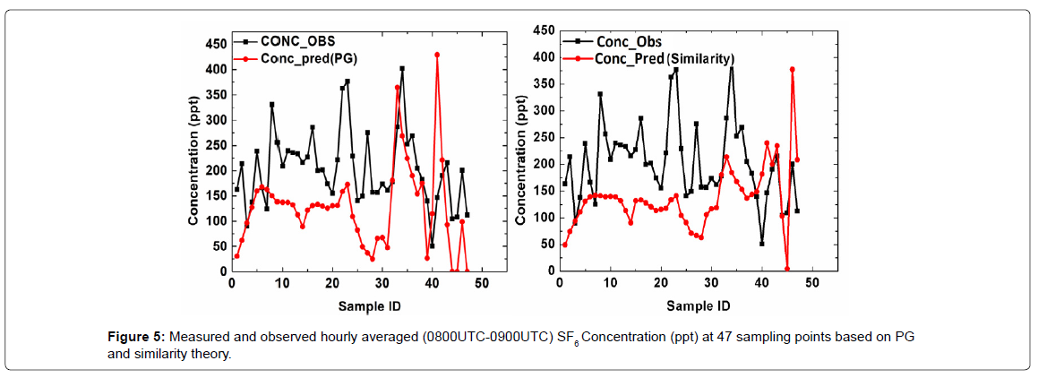
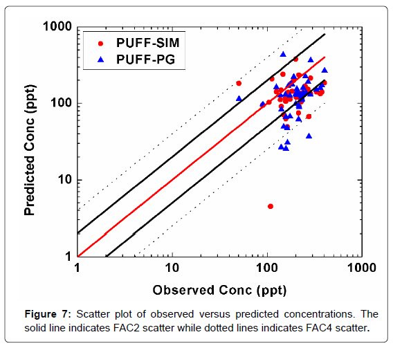
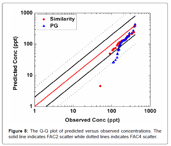
In order to study the sensitivity of CALPUFF model to selection of the dispersion coefficient, two numerical simulations were performed to investigate the CALPUFF performance using dispersion coefficients based on PG curves and those based on similarity theory. Figure 5 shows the hourly averaged observed and simulated SF6 concentration at discrete sampling points by choosing PG dispersion coefficient and dispersion coefficient based on similarity theory. The model underestimates at most of the sampling points, however it is seen that both observed and predicted concentrations follow the same trend in shape and magnitude. The results show that the dispersion coefficients based on similarity theory perform better in such conditions than PG dispersion coefficients. Concentrations contours through interpolation were plotted using the values at discrete sampling points to show comparison of spatial distribution of predicted and observed concentrations. The model accurately predicted the position and direction of plume. However, the horizontal extent of plume and central maximum concentration were under-estimated in downwind direction away from the source as shown in Figure 6. The plume shows non-homogeneous (non-Gaussian) distribution of concentrations due to complex terrain. Hourly averaged measured and predicted concentrations were used to perform statistical analysis of model performance. The statistical indices namely FB, NMSE, FAC2, FAC4, and FOEX showed good performance of model in simulating the dispersion of tracer in near field complex terrain. The statistical indices indicated that CALPUFF model with choice of dispersion coefficients based on similarity theory performed better than dispersion coefficients derived from PG curves. The fractional bias (-0.39) indicates underprediction of CALPUFF model with similarity dispersion coefficients. The NMSE has a low value of 0.43 reflecting lower scatter of predicted data around the observations. FAC2 and FAC4 have values of 68.08% and 95.74% reflecting good agreement between predicted and observed concentrations. The FOEX has a value of -28.72%, which shows more under-prediction than over-predictions (Table 5).The performance of CALPUFF model using different dispersion coefficients was also investigated using scatter and Quantile-quantile (Q-Q) plot. In scatter plot, the paired observed and predicted concentrations are plotted against each other which qualitatively give measure of underprediction or over-prediction. If the atmospheric dispersion model is intended to be used for operational purposes, then its compliance to air quality regulations is determined. For this purpose the highest short-term concentrations are studied for potential Exceedance from threshold values irrespective of time and location (Chang et al., 2005). The Q-Q plot gives a measure of how closely the predicted concentration distribution is following the observed one especially for high concentration values. The Q-Q plot is created by first sorting the predicted and observed concentrations by rank and then plotting the quantiles against each other. In Q-Q plot the predicted and observed concentrations are no longer paired in time or space (U.S. EPA).As shown in Figure 7, at higher concentrations the predicted values are relatively close to the observed concentrations lying within FAC2 lines. For dispersion coefficients based on similarity theory most of the points are within FAC2 range and almost all the points are in FAC4 lines. The Q-Q plot gives visual representation for under-prediction and over-prediction and shows how closely the predicted distribution is following the observed distribution. The Q-Q plot (Figure 8)shows that the model strongly under-predicts at lower concentration and starts to perform better at higher concentrations. Over most of the plotting range, the similarity method shows less bias (under-prediction) as compared to PG method.
| Statistical test | PG | Similarity |
|---|---|---|
| Fractional Bias | -0.46 | -0.39 |
| NMSE | 0.51 | 0.43 |
| FAC2 | 51.06 | 68.08 |
| FAC4 | 85.11 | 95.74 |
| FOEX | -32.98 | -28.72 |
Table 5: Statistical indices for model performance evaluation.
Conclusion
A tracer experiment was performed to test the performance of CALPUFF model in near field complex terrain for short-term shortrange release scenarios. The model was configured and optimized in real time meteorological and topographical conditions of Pakistan. High temporal and spatial resolution of meteorological input was used, which enabled the CALMET model to simulate properly the small scale variation in the wind field. CALMET model was optimized using different options for grid resolution, land use dataset and temporal resolution ofmeteorological input.The best resultswere achieved forthe grid resolution of 300 m, SRTM3 dataset and 5 minutes meteorological data input. The impact of selecting dispersion method on ground level concentrations calculation was investigated. Two numerical simulations were performed to investigate the CALPUFF performance using dispersion coefficients based on PG curves and those based on similarity theory. In short-range short-term dispersion phenomenon, prediction of concentration was found to be dependent upon selection of dispersion coefficients. The dispersion coefficients based on similarity theory performed better than dispersion coefficients derived from PG curves in complex terrain setting. It was found that CALPUFF in near field complex terrain and short term release scenario underestimates the tracer concentrations. However, according to statistical indices, overall the observed and the predicted concentrations were in good agreement for this field tracer test.
References
- De Visscher A. Air dispersion modeling: foundations and applications. John Wiley & Sons; 2013 Sep 26.
- Barclay J, Scire J. Generic Guidance and Optimum Model Settings for the CALPUFF Modeling System for Inclusion into the “Approved Methods for the Modeling and Assessments of Air Pollutants in NSW. Australia, Atmospheric Studies Group, TRC Environmental Corporation, Lowell. 2011.
- Steyn DG, Chaumerliac N, editors. Air Pollution Modeling and Its Application XXII. Springer; 2014 May 9.
- Lee HD, Yoo JW, Kang MK, Kang JS, Jung JH, et al. Evaluation of concentrations and source contribution of PM10 and SO2 emitted from industrial complexes in Ulsan, Korea: Interfacing of the WRF–CALPUFF modeling tools. Atmospheric Pollution Research. 2014; 1;5:664-76.
- Schramm J, Degrazia FC, Vilhena MT, Bodmann BE. Comparison of CALMET and WRF/CALMET coupling for dispersion of NO2 and SO2 using CALPUFF modelling system. American Journal of Environmental Engineering [recurso eletrônico]. Rosemead. 2016;6;4,50-55.
- Oleniacz R, Rzeszutek M. Intercomparison of the CALMET/CALPUFF modeling system for selected horizontal grid resolutions at a local scale: a case study of the MSWI Plant in Krakow, Poland. Applied Sciences. 2018;8:2301.
- Yao R, Xu X, Xin C. A tracer experiment study to evaluate the CALPUFF real time application in a near-field complex terrain setting. Atmospheric Environment. 2011; 1;45:7525-32.
- Zuas O, Budiman H, Hamim N. Measurement of SF6 using gc-ecd: a comparative study on the utilization of CO2-N2 mixture and CH4-Ar mixture as a make-up gas. Chemistry & Chemical Technology, 4, 2017.
- Lim JS, Moon DM, Kim JS, Yun WT, Lee J. High-precision analysis of SF 6 at ambient level. Atmospheric Measurement Techniques. 2013 ; 5;6:2293-9.
- Lim JS, Moon DM, Kim JS, Yun WT, Lee J. High-precision analysis of SF 6 at ambient level. Atmospheric Measurement Techniques. 2013 ; 5;6:2293-9.
- Farr TG, Rosen PA, Caro E, Crippen R, Duren R, et al. The shuttle radar topography mission. Reviews of geophysics. 2007 ;45.
- Chang JC, Hanna SR. Technical descriptions and user’s guide for the BOOT statistical model evaluation software package, version 2.0. George Mason University and Harvard School of Public Health, Fairfax, Virginia, USA. 2005 Jul 10.
- Zhu H, Li F. Evaluation of algorithms of dispersion coefficients with a field tracer experiment over complex terrain. InInternational Confernece Pacific Basin Nuclear Conference 2016 ;5 ;473-485.
- Chang JC, Hanna SR. Air quality model performance evaluation. Meteorology and Atmospheric Physics. 2004;87:167-96.
- Hanha SR. Air quality model evaluation and uncertainty. Japca. 1988; 1;38:406-12.
Citation: Amin ul H, Qaisar N, Amjad F, Naseem I, Masroor A, et al. (2021) Sensitivity Analysis of CALPUFF Model: Application Over Complex Terrain. J Earth Sci Clim Change 12: 559. DOI: 10.4172/2157-7617.1000559
Copyright: © 2021 Amin ul H, et al. This is an open-access article distributed under the terms of the Creative Commons Attribution License, which permits unrestricted use, distribution, and reproduction in any medium, provided the original author and source are credited.
Select your language of interest to view the total content in your interested language
Share This Article
Recommended Journals
Open Access Journals
Article Tools
Article Usage
- Total views: 4275
- [From(publication date): 0-2021 - Nov 12, 2025]
- Breakdown by view type
- HTML page views: 3227
- PDF downloads: 1048

