Analysis of Ground Level O3 and Nox Measured at Kannur, India
Received: 11-Apr-2012 / Accepted Date: 25-May-2012 / Published Date: 28-May-2012 DOI: 10.4172/2157-7617.1000111
Abstract
This paper presents the observations of continuous measurements of surface Ozone (O3) and Oxides of Nitrogen (NOx) present in the ambient air over Kannur University Campus (11.9º N, 75.4º E, 5m), Kerala State, India from November 2009 to October 2010. The diurnal cycle of surface O3 concentration exhibited a peak in the afternoon and declined during nighttime on all days of observation. Likewise, the annual average diurnal variation of O3 mixing ratio showed a minimum of (3.2 ± 0.7) ppbv in the morning and a maximum of (30.3 ± 10.4) ppbv at noon. The highest mixing ratios of surface O3 observed during winter and summer at this site were 44 ppbv and 33.4 ppbv respectively and that during the monsoon and post-monsoon seasons were 18.5 ppbv, and 28 ppbv respectively. The diurnal profile of NOx (NO+NO2) showed a peak during the early morning hours and decreased during the noontime. Correlations between O3 with NO, NO2 and NOx with NO, NO,sub>2 has discussed in detailed. The concept of total oxidant, OX (O3+NO2) has been introduced, and found to vary with the level of NOx. The influence of relative humidity and temperature on the variation in O3 is discussed. The variations of O3 in different months were elucidated with the aid of backward air trajectories of CGER-METEX reanalysis data.
Keywords: Surface ozone; Photochemical production; NOx ; Oxidant; Air quality
5470Introduction
Air pollution will be an important and challenging problem in the coming decades that will affect sustainable development of nations [1-3]. The rapid growths in industrial activities due to globalization result in vast amounts of potentially harmful gases and particles being emitted into the atmosphere on a global scale [4]. Prominent air pollutants are sulphur compounds (SO2 and H2SO4) nitrogen compounds (NOx and NH3), carbon monoxide (CO) and organic compounds (hydrocarbons, VOCs, halogenated compounds). These trace gas species in the atmosphere produce other secondary pollutants via thermal, chemical and photochemical pathways [5,6]. Surface O3 is identified as one of the air pollutants that effect human health and the ecosystem [7-9]. Surface level O3 concentration has steadily increased since the 19th century [10,11]. The sources of surface O3 are in-situ photochemical production, transport from other in-situ production sites and downward transport from the stratosphere [12-15].
The photochemical production of O3 is enhanced by the chemistry involving CO, CH4, Non-Methane Hydro Carbons (NMHC) and other Volatile Organic Compounds (VOC) and occurs in the presence of sufficient amount of NOx and depends on the concentrations of hydroxyl and other radicals which act as catalysts [16-21]. NOx and VOCs are emitted from anthropogenic sources such as fossil fuel combustion, power plants, industrial activities and transportation, as well as from natural sources such as lightning, and vegetation (biogenic VOCs such as isoprene). Recently, elevated concentrations of O3 have been observed even over large rural areas in developed countries due to anthropogenic activities and biogenic emissions where industrial activities are limited [22-26]. Two mechanisms have been proposed to account for the high rural O3 [27-29]. One is the transport of O3 from urban areas, and the other is the transport of its precursors like NOx and non-methane hydrocarbons [30], followed by photochemical O3 production. Ozone is a strong oxidizer in the atmosphere and its chemistry is complex. However, the relationship between O3 and its precursors represents one of the major scientific challenges associated with urban air pollution [31,32]. Further, O3 being a strong greenhouse gas, increasing levels of O3 can warm the troposphere, and induce significant changes in the climate over an extended period of time [33,34]. Thus, a long-term investigation of surface O3 and its precursors is essential to understand the ambient air quality over a location. Meteorological parameters including wind speed, wind direction, temperature, solar radiation and relative humidity have substantial influences on O3 concentrations [35,36]. Generally, O3 is observed to be higher in both winter and summer at many measurement sites over the globe [37].
Surface O3 in the atmosphere has been monitored sporadically at various sites around the globe for the past several decades [38,39] Many studies have been carried out on the photochemical characteristics of O3 and its precursor gases in the United States [40,41] and most networks in Europe were implemented at the beginning of 1980s. Atmospheric concentrations of O3 and its precursors like NOx and VOCs are increasing rapidly in Southeast Asia as a result of the fast growth of the transportation and industrialization [42] found that the transport sector contributed 37% of the NOx emissions, while 27% came from power generation and 18% from industry. Measured and modeled O3, NOx and VOCs in Shanghai, China by [43] shows that O3 concentrations are higher in rural area than in center of the city, suggesting that there are O3 depression processes in center of city and air pollutant emissions are not favorable for the O3 chemical formation. The studies on the significant role of O3 influenced on the ambient air quality were reported by [44,45]. Further [46] found that Surface O3 at a coastal site in Hong Kong is strongly influenced by the outflow of Asian continental air during the winter and the inflow of maritime air from the subtropics in the summer. Modeling studies have been emerged as one of the promising methods to evaluate the production and transport of O3 confined in a region. Such studies were carried out by many groups [47-50] which were quite promising.
In the Indian continent, available observations [51-54] and modeling studies [32,55] show higher O3 levels during spring winter and summer extending until May. Such variations over India are due to higher levels of precursors and the availability of abundant solar radiation flux during these seasons. In India, various groups have been involved in carrying out long-term measurements of surface O3 and its precursors; their observations are quite relevant in understanding the regional air quality [28,32,45,52,56-66]. In order to explore O3 chemistry and its transport at Kannur, a tropical coastal site in the state of Kerala in India, a continuous observation has been on-going with the support of Atmospheric Chemistry Transport and Modelling (AT-CTM) project under Geosphere Biosphere Programme (GBP) of the Indian Space Research Organization (ISRO). This study describes the key observations of both seasonal and diurnal variations of surface O3 and its precursor NOx and their variations with meteorological parameters. The location is rural with limited industrial activities. The observation of ambient air quality over this location for a period of one year from November 2009 to October 2010 revealed that the seasonal variation of O3 was influenced by meteorology and air mass movement. This manuscript begins with a brief introduction.
Methods
Monitoring site
The location of the sampling site at Kannur University campus (KUC) (11.9°N, 75.4°E 5m) is shown in Figure 1. Observation site is in the northern part of Kannur district in Kerala state which is surrounded on one side by a river basin and the other side by the Arabian Sea. This site is in the valley of the mountains of Western Ghats. It is a rural location with no major industrial activities except a few small-scale industries such as plywood and mattress manufacturing units. The distance to the seashore to the west is 4 km and that to the Western Ghats on the east is 50 km. The land area of Kannur is about 3000 km2 with an average population density of 1000 per km2. KUC is situated in an open land which receives plenty of sunshine (peak average of 1 ± 0.3 KWhr/m2) throughout the day, and the land is surrounded with green vegetation throughout the year.
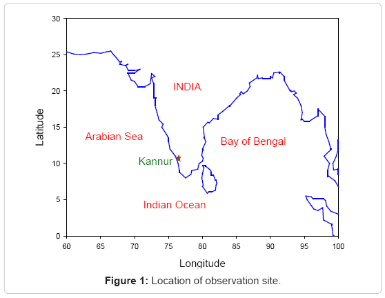
Figure 1: Location of observation site.
Meteorological background
A prominent meteorological characteristic of this location is the intense monsoon rainfall occurring in two spells every year. The southwest monsoon is active during the months of June-August, and this intense rainfall has been classified as the Monsoon Season. This is followed by the return monsoon or northeast monsoon in November. Hence September, October and November are earmarked as the post monsoon (autumn) season with scattered showers accompanied by heavy thunder and lightning. The intensity of summer is masked by the southwest monsoon season over the entire region. About 80% of the total rainfall occurs from June to August which constitutes the main monsoon season. The months, December, January and February with scant rainfall and relatively low humidity constitute the winter season. From March to May the season is summer with scorching heat and high convective flow. Thus, we have Easterly wind during winter months from December to February, the Westerly and South-Westerly winds during summer, and the monsoon and post-monsoon season. The period from January to March records the maximum sunshine hours of more than 9.1 hours/day and between June and August records the minimum sunshine due to cloudy skies. Figure 2 shows the monthly variations of meteorological (wind speed, temperature, relative humidity and rainfall) in Kannur during the period of observation. The temperature was high between March and May and was low during June through August. The average monthly high temperature ranged from 29.6 to 37.1°C and low temperature ranged from 22.9 to 25.8°C.
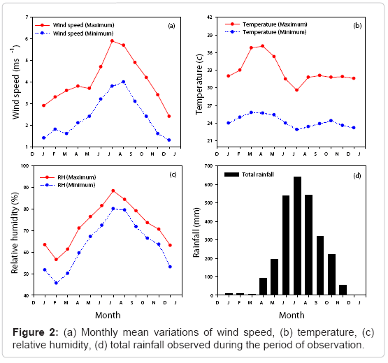
Figure 2: (a) Monthly mean variations of wind speed, (b) temperature, (c) relative humidity, (d) total rainfall observed during the period of observation.
The maximum humidity was measured during monsoon (June, July, August) and minimum was observed during winter months (December, January, February). The maximum monthly average relative humidity ranged from 55.5% to 88.4% and minimum of 45% to 80% at this location. The maximum rainfall was recorded during monsoon, while minimum was observed during the winter season. Figure 3 shows the monthly mean wind speed and wind direction at 1000 hPa during the study period at the observation site. The wind speed is steady during monsoon season and minimum during winter season. It was pretty high during the period from June to September and low from December to April. The maximum average wind speed ranged from 2.4 to 5.9 km per hour and the minimum from 1.3 to 4 km/hr during the period of observation.
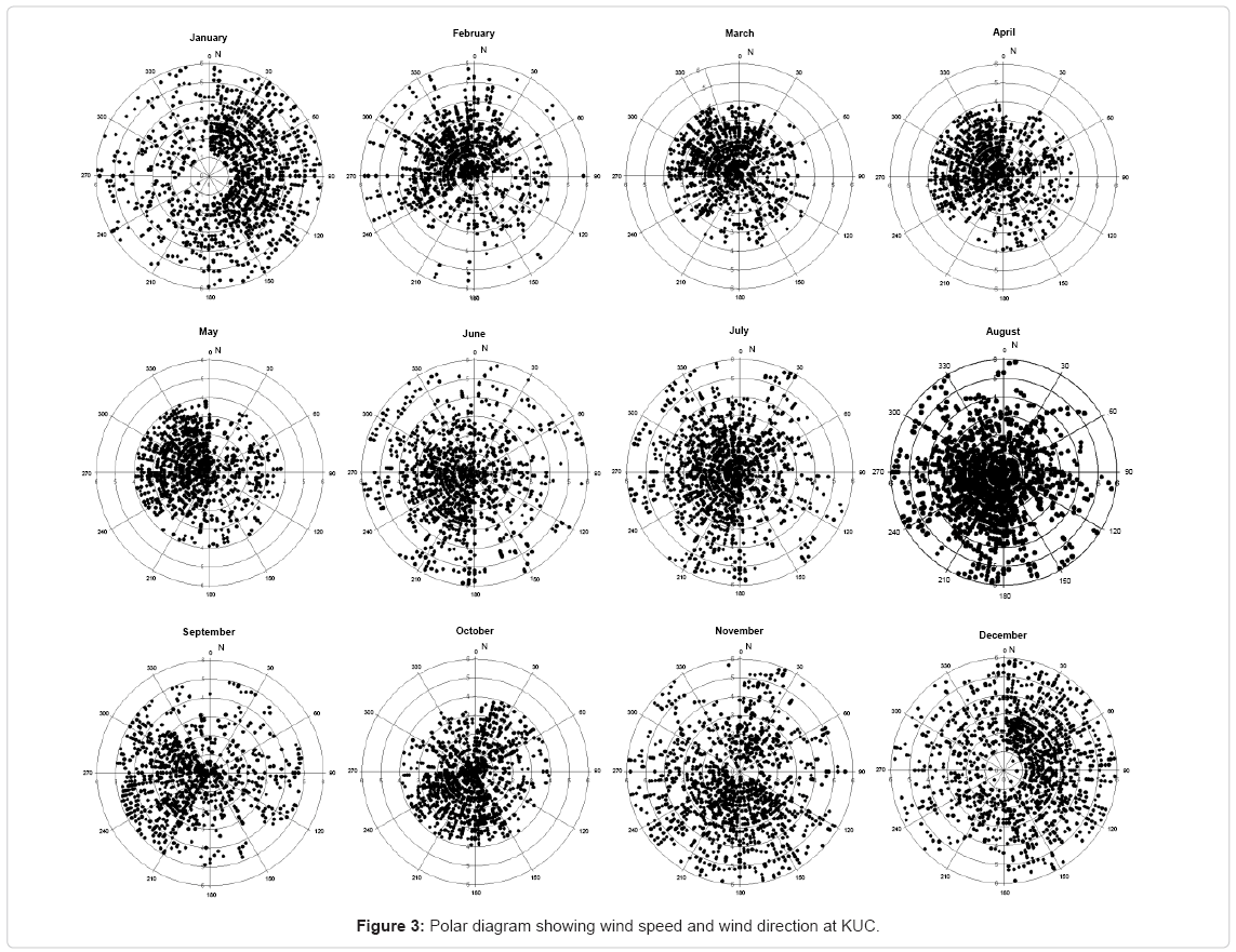
Figure 3: Polar diagram showing wind speed and wind direction at KUC.
The meteorological parameters like temperature, relative humidity, wind speed and wind direction were collected from the local automatic weather station, which is one of the stations managed by the Meteorological and Oceanographic Satellite Data Archival Centre (MOSDAC) and established by the Indian Space Research Organization (ISRO).
Measurement techniques
The concentrations of surface O3 and NOx were measured simultaneously with the aid of respective gas analyzers from Environment S.A., France. The ambient air collecting sampling inlet hood was placed at a height of 6 m from the ground and data were continuously recorded from November 2009. The concentrations of O3 were obtained using the ozone analyzer (Model O3 42M) and the details of the analyzer and its principle were described elsewhere [67-69] Calibration of the analyzer was performed at regular intervals using ozone free air and pure ozone produced by the appropriate gas generators in the analyzer. It has a lower detectable limit of 0.4 ppbv with a minimum response time of 20 seconds. This analyzer is provided with an in-built correction for temperature and pressure variations as well as intensity fluctuations of the light source. Similarly total NOx was monitored with the aid of a standard chemiluminescent analyzer (Model AC32M). The method was found to have higher sensitivity and specificity [70-72]. The lower detectable limit was 0.4 ppbv with a response time of 30s. The calibration of the analyzer was carried out using reference gas cylinders.
Results and Discussion
Diurnal variation of ozone
Eight hour averaged (09:00-17:00 h) surface O3 concentration measured from November 2009 to October 2010 on a day-to-day basis is shown in Figure 4. Despite considerable short-term variations, a seasonal change was seen for the entire period. Among the maximum mixing ratio of O3, eight-hour average highest and lowest values were observed in December (46.9 ppbv) and in July (16.4ppbv). From the Figure 4, it is clear that O3 levels were observed to be the highest in winter and lowest during the monsoon season.
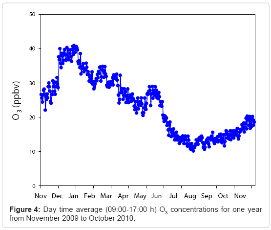
Figure 4: Day time average (09:00-17:00 h) O3 concentrations for one year from November 2009 to October 2010.
The enhanced O3 mixing ratio observed during winter season was mainly due to the easterly air flow that favours advection of precursors from inland locations which induces active photochemistry. Figure 5 shows the diurnal variation of O3 for different months over a period of one year from November 2009 to October 2010. The vertical bars shown in the Figure 5 are 1σ standard deviation. The highest maximum O3 concentration was observed in December and minimum in July.
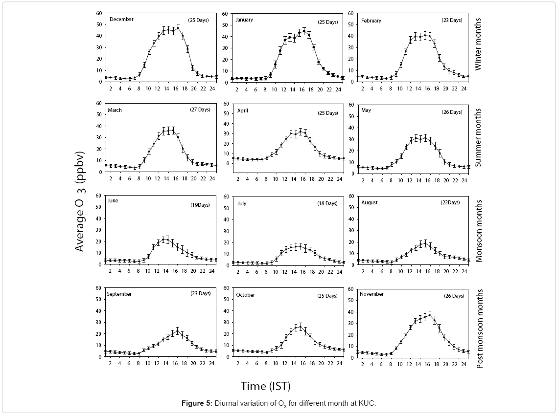
Figure 5: Diurnal variation of O3 for different month at KUC.
The daytime increase in O3 mixing ratio is mainly from the photo-oxidation of industrial and anthropogenic hydrocarbons, carbon monoxide, and methane in the presence of sufficient amount of NOx [58,73,74] With the onset of sunshine, O3 concentration gradually increases and it reaches a maximum value at 14:00 h noontime, due to its photochemical formation through the photolysis of NO2 via the following set of reactions.
NO2 + hν (λ< 420 nm) →NO + O (R1)
O + O2 + M → O3 + M (R2)
It was observed that the mixing ratio of O3 started to decline after 16:30 h in the evening on all days. The low concentration of O3 observed during nighttime is due to the absence of photolysis of NO2 and loss of O3 by NO through the following titration reaction and surface deposition.
O3+ NO → NO2 + O2 (R3)
Loss of O3 also occurs due to both dry and wet deposition that results in a minimum concentration at sun rise. [28] Have observed a similar diurnal variation at Gadanki, a rural site in south-east India (13.5°N, 79.20E, 375m asl). To substantiate the annual surface O3 variation, seasonal average daytime, nighttime O3 mixing ratios and the rate of change during morning and evening are presented in (Table 1).
| Month | Average O3 (20:00- 08:00 h) ppbv |
Average O3 (08:00-20:00 h) ppbv |
O3 minimum (ppbv) | O3 maximum (ppbv) | Rate of increase (08:00-11:00 h) ppbv/h |
Rate of decrease (17:00-19:00 h) ppbv/h |
|---|---|---|---|---|---|---|
| January | 4.4 ± 2.0 | 29.3 ± 4.3 | 2.8 | 44.6 | 8.2 | -11.9 |
| February | 4.7 ± 1.9 | 26.5 ± 4.2 | 3.0 | 40.6 | 7.5 | -10.0 |
| March | 5.2 ± 1.8 | 22.6 ± 3.9 | 3.5 | 36.1 | 6.6 | -5.9 |
| April | 4.9 ± 1.8 | 20.1 ± 3.8 | 3.9 | 31.9 | 4.2 | -6.2 |
| May | 5.7 ± 1.9 | 21.5 ± 4.1 | 4.5 | 31.2 | 5.2 | -7.0 |
| June | 3.6 ± 1.2 | 13.0 ± 3.4 | 2.5 | 21.4 | 4.1 | -2.4 |
| July | 2.8 ± 1.2 | 11.0 ± 3.4 | 1.9 | 16.4 | 2.9 | -3.0 |
| August | 4.1 ± 1.3 | 11.3 ± 3.4 | 2.3 | 18.6 | 2.4 | -2.7 |
| September | 4.3 ± 1.4 | 13.5 ± 3.4 | 2.6 | 22.4 | 2.2 | -3.3 |
| October | 5.5 ± 1.4 | 15.2 ± 3.6 | 3.7 | 26.1 | 2.0 | -3.5 |
| November | 5.2 ± 1.5 | 24.4 ± 3.9 | 2.9 | 37.1 | 5.3 | -7.5 |
| December | 4.1 ± 2.0 | 31.9 ± 4.7 | 2.7 | 46.9 | 9.2 | -14.0 |
Table 1: Monthly average daytime and night time O3, maximum and minimum O3 and the rate of change of O3 at KUC.
From the Table 1, it is evident that the observed higher O3 mixing ratios were in December (46.9 ppbv) while lower mixing ratios were in July (16.4 ppbv). This may be due to the variations in precursor gases and the influence of changing meteorological parameters. The daytime high average O3 mixing ratio observed in December (31.9 ± 4.7) ppbv was due to the lower boundary layer that occurs in winter and the low relative humidity. The daytime low average O3 mixing ratio was in July (11.0 ± 3.4) ppbv, which is mainly due to the intense southwest monsoon which removes pollution over this location. The highest rate of O3 increase (9.2ppbv/h) was observed in December between 08:00-11:00 h Indian Standard Time (IST) and lowest (2.4ppbv/h) was found in August. The O3 removal rate was the highest in December (-14.0ppbv/h) between 17:00-19:00 h IST and the lowest was in June (-2.4ppbv/h).
Seasonal variation of O3
Figure 6 shows the seasonal average diurnal variation of O3 during 2009-2010 at KUC. The variations in O3 concentrations for different seasons namely winter (DJF), summer (MAM), monsoon (JJA) and post-monsoon (SON) are shown. It is observed that the variation of O3 during all seasons shows a similar pattern. Among the maximum concentration, the highest value of O3 mixing ratio was found in winter (44 ± 3.1) ppbv and the lowest during the monsoon season (18.46 ± 3.5) ppbv. The lowest magnitudes of O3 mixing ratios observed were (4.0 ± 1.4) ppbv in summer and (2.24 ± 1.26) ppbv in monsoon seasons. The highest O3 observed in winter is attributed to a lower mixing height that results in trapping of pollutants near the earth’s surface due to temperature inversion [25]. Similar patterns of seasonal variations have also been observed at Gadanki [28] Anantapur [75] and Trivandrum [66] in south India. The minimum and maximum mixing ratios of O3 found at this site during monsoon were (2.3 ppbv, 18.5 ppbv) and post monsoon were (3.3 ppbv, 28.0 ppbv) respectively. From this it is evident that O3 exhibits a distinct seasonal variation over this site, which may not only be controlled by solar radiation, but also by atmospheric dynamics as well. There is also a possibility of enhanced transport of O3 from the stratosphere during the winter season [64,74]. Further the active photochemistry of NOx under clear sky conditions in winter season would enhance the O3 abundance.
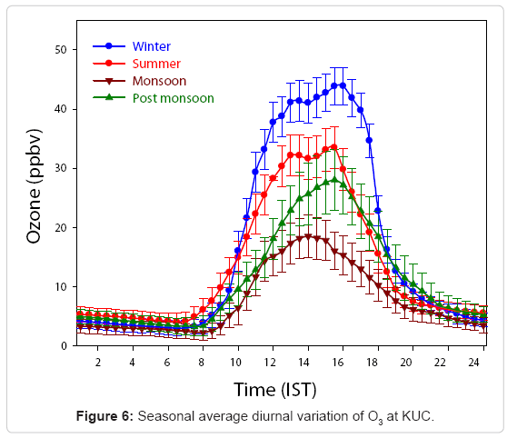
Figure 6: Seasonal average diurnal variation of O3 at KUC.
This in turn offers a suitable environment for the production of added O3 during winter season at this site. Moreover, the meteorological parameters have a strong influence on the seasonal changes in the concentration of O3. An enhancement in the boundary layer height and increased cloud cover over this location during summer induce a relatively small mixing ratio observed in summer than in winter. A relatively low amount of surface O3 was observed during monsoon seasons than summer and winter seasons. During the monsoon period, the absence of sunshine and high relative humidity reduce the O3 concentration at this location. Seasonal average variations of O3 during day time and night time are shown in (Table 2).
| Season | Average O3 (20:00-08:00 h) ppbv |
Average O3 (08:00-20:00 h) ppbv |
O3minimum (ppbv) | O3 maximum (ppbv) |
|---|---|---|---|---|
| Winter | 4.4 ± 1.9 | 29.2 ± 4.4 | 2.9 | 44.0 |
| Summer | 5.3 ± 1.8 | 21.4 ± 3.9 | 4.1 | 33.4 |
| Monsoon | 3.5 ± 1.2 | 11.8 ± 3.4 | 2.3 | 18.5 |
| Post monsoon | 4.9 ± 1.4 | 17.7 ± 3.6 | 3.3 | 28.0 |
Table 2: Seasonal average day and night time O3, maximum and minimum O3.
From the Table 2, it is clear that daytime average O3 concentration became a maximum (29.2 ±4.4) ppbv during winter while nighttime O3 became higher during summer (5.3 ±1.8) ppbv due to the land air mass influence in winter and oceanic influence in summer as observed from the backward trajectory depicted in of Air trajectories during the period of observation. The minimum and maximum observed mixing ratios of O3 during winter were 2.9 ppbv, 44.0 ppbv and that during summer was 33.4ppbv, 4.1 ppbv respectively. From this it is evident that O3 variation is not only controlled by solar radiation, but also by atmospheric dynamics. The favorable conditions for photochemical production of O3 are satisfied at KUC during winter months. Moreover, the meteorological parameters have a strong influence on the seasonal changes in the concentration of O3. A relatively small mixing ratio observed in summer than in winter is due to high air temperature induced convective activities and increased cloud cover. The minimum and maximum observed mixing ratios of O3 during monsoon were 2.3 ppbv, 18.5 ppbv and that for post monsoon were 3.3 ppbv, 28.0 ppbv respectively.
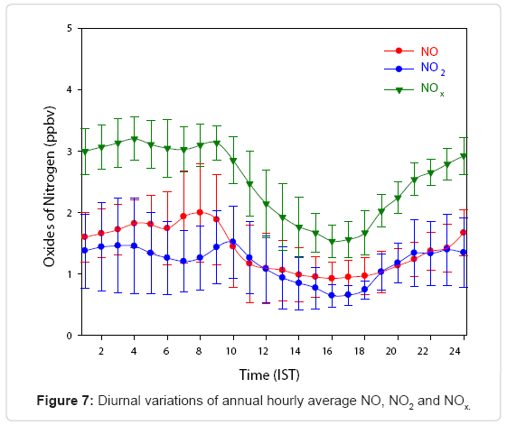
Figure 7: Diurnal variations of annual hourly average NO, NO2 and NOx.
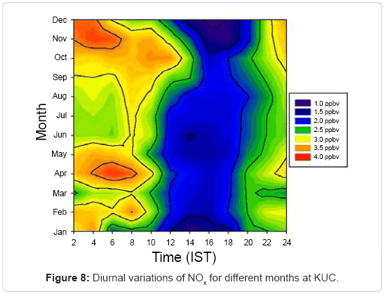
Figure 8: Diurnal variations of NOx for different months at KUC.
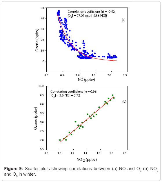
Figure 9: Scatter plots showing correlations between (a) NO and O3 (b) NO2 and O3 in winter.
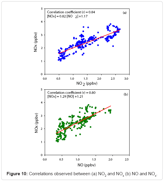
Figure 10: Correlations observed between (a) NO2 and NOx (b) NO and NOx.
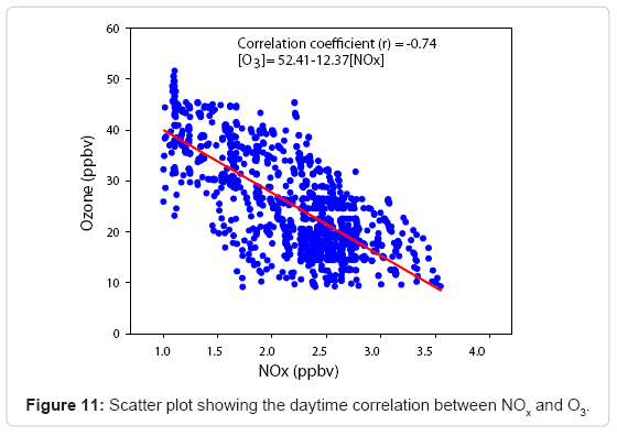
Figure 11: Scatter plot showing the daytime correlation between NOx and O3.
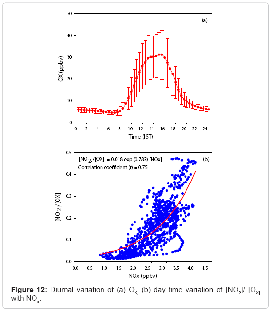
Figure 12: Diurnal variation of (a) OX, (b) day time variation of [NO2]/ [OX] with NOx.
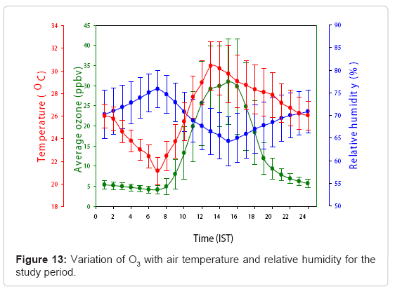
Figure 13: Variation of O3 with air temperature and relative humidity for the study period.
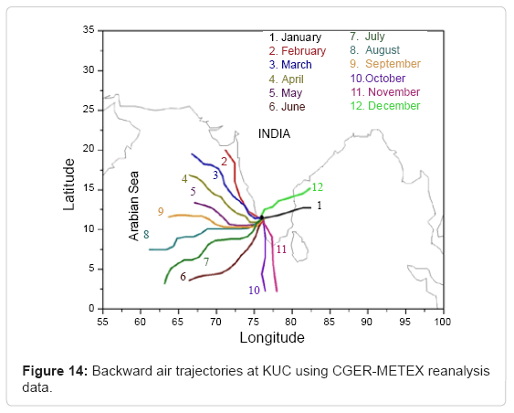
Figure 14: Backward air trajectories at KUC using CGER-METEX reanalysis data.
Diurnal and seasonal variations of NO, NO2 and NOx
Figure 7 shows the annual average diurnal variations of NO, NO2 and NOx observed at KUC. The morning peak of NO2 appears 2h after the NO peak. Subsequently, after the morning peak, NO diminishes until it reaches its lowest value at 15:00 h and has a gradual increase till midnight. During nighttime, surface emission of NO were limited inside the nocturnal planetary boundary layer, and NO reached its second highest peak at midnight. Likewise, a decline in NO2 mixing ratio observed during daytime was due to the enhanced photolysis by which O3 is formed at this site. It was observed that NOx mixing ratio started declining from (3.1 ± 0.28) ppbv at 09:00 h IST and it became a minimum of (1.53 ± 0.26) ppbv at 16:00h and began to regain in magnitude during nighttime. This reduction in NOx concentration boosts the production of O3 through photolysis induced by sunlight in daytime. At night, the relatively low air temperature near the surface could prevent the vertical dispersion of NOx, contributing to its accumulation and resulting in high nighttime mixing ratio. Higher levels of NOx during early morning and night hours are due to the combination of anthropogenic emissions, boundary layer processes, chemistry as well as local surface wind pattern [28,75]. During nighttime, the boundary layer descends and remains low till early morning, hence pollutants get trapped in the shallow surface layer and show higher concentration. In order to attain high levels of O3 during noon, large amounts of precursors are needed, and this may leads to low levels of NOx during daytime [57].
At this site, the annual average mixing ratio of NOx is found to be about 2.5ppbv, which is relatively small compared to that of rural sites, where mixing ratios can be much higher [28]. The diurnal variation of NOx for different months is shown in Figure 8. The maximum and minimum concentrations of NOx observed at KUC were (3.9 ± 0.5) ppbv and (1.0 ± 0.3) ppbv in December and January respectively. The maximum rate of change of NOx occurs in December in which O3 concentration is high and the minimum rate is in July in which O3 concentration is lowest.
The maximum magnitudes of average NOx concentration (2.9 ± 0.8) ppbv were observed in summer and minimum during monsoon (2.3 ± 0.4) ppbv. During winter the maximum average concentration was (2.5 ± 0.6) ppbv and post-monsoon it was (2.7 ± 0.7) ppbv. Thus the concentration of NOx did not show significant variation during the period of observation at this site but only had a small seasonal variation. NOx mixing ratios are generally stronger during early morning and nighttime in all the seasons. The minimum and maximum observed mixing ratios of NOx were 1.3 ppbv, 3.5 ppbv (winter), 1.6 ppbv, 3.3 ppbv (summer), 1.6 ppbv, 3.2 ppbv (monsoon) and 1.5 ppbv, 3.4 ppbv (post monsoon).
Analysis of O3, NO, NO2 and NOx
The basic process leading to the photochemical formation of O3 in the lower troposphere and the polluted urban atmosphere involves the photolysis of NO2 to yield NO and a ground-state oxygen atom. O3 is formed and destroyed in a series of reactions involving NO and NO2 as described by (R1), (R2) and (R3) in Diurnal variation of ozone where M denotes a third body like a nitrogen or oxygen molecule that absorbs the excess vibrational energy and eventually stabilizes the O3 molecule thus formed. In the absence of other chemical species, these three reactions govern O3 concentration. Figure 9 (a) represents the variation of O3 concentration with NO mixing ratio within a sample interval of 15 minutes. It is evident that O3 concentration diminishes as NO mixing ratio increased, which may be due to the removal of O3 by titration with NO. The most appropriate fit to this distribution is exponential and the empirical relation is (Figure 9)
[O3] = 97.07 exp (-2.36 [NO]) (1)
Thus, a fast decay in O3 concentration is observed at high NO mixing ratios from late evening to early morning. Further, the daytime variation between O3 and NO2 observed on the maximum number of clear sky days available during winter mornings is shown in Figure 9(b). A linear fit with excellent correlation with a significance level (p < 0.01) that occurs in the winter season reveals the active photochemistry of O3 production, which starts early morning. The empirical relationship observed between [O3] and [NO2] is
[O3] = 3.6[NO2] + 3.72 (2)
Figure 10 (a) represents the variation of NO2 and NOx using the mean observed data. A linear fit with a good correlation is obtained and the observed empirical relationship is
[NOx] = 0.82[NO2] + 1.17 (3)
and it shows the active competition between NO2 and NOx on the chemistry of O3 at this location.
The correlation between NO and NOx shown in Figure 10 (b) which yields a linear relationship with an empirical relation
[NOx] = 1.29[NO] + 1.21 (4)
and this enhanced influence of NO mixing ratio is the primary reason for the nighttime reduction in O3 concentration at this site. However, the wet and dry depositions of O3 to land and marine surfaces are significant due to the proximity of Arabian Sea and with fairly good vegetation in the area. Figure 11 shows a negative linear correlation between daytime O3 and NOx observed during the whole period of observation suggesting the possible VOC-sensitive characteristics of the study location as described by [76,77] and the linear relation is as
[O3]= 52.41-12.37 [NOx] (5)
The coefficient of this correlation is -0.74, which is quite significant.
The organic emissions from nearby wetlands and biogenic VOCs from vegetation make this location VOC sensitive assuming that the higher O3 levels appear when the VOC concentrations increase. Fishing boats and ship emissions are other strong contributors of organic species over the Arabian Sea [78]. The significant contribution to NO2, SO2, Black Carbon (BC) and Organic Compounds (OC) is large over coastal zones. Secondary species formed from fishing boat emissions have large chemical lifetimes and are transported in the atmosphere over several hundreds of kilometers. Thus, they can contribute to air quality problems on land [79]. In general, the emission perturbation is most effective in increasing ozone formation over regions with low background pollution [19]. The region in the sea which is adjacent to our sampling location is an estuary with a good catchment area. The marine department of the state of Kerala has estimated that approximately 1425 fishing boats are engaged in fishing from early morning 06:00 h to 14:00 h on all days in a span of 4 km from the shore of the Arabian Sea in Kannur region except during the monsoon season. It is estimated that about 8 liters of diesel is consumed per hour by a single vessel and on an average 16 kilolitres of diesel is burnt per day. The sea breeze at noon time transports these organic compounds from the sea to the land. PM10 samples have been collected using a Respirable Dust High Volume Air Sampler (ENVIROTECH, India Model APM 460 NL) at this site and the chemical analysis employing gas chromatography revealed the presence of several organic species during the day time and is listed (Table 3).
| Aliphatic compounds and derivatives |
Pentane, 2,3,3 –trimethyl- |
| Heptane, 3,3,5- trimethyl- | |
| Nonadecane | |
| Octane, 2,6-dimethyl- | |
| Octane, 2,3-dimethyl- | |
| Octane, 3,3-dimethyl- | |
| Octadecene | |
| Dodacane, 2,6,111-trimethyl- | |
| Tetradecene | |
| Tetrapentacontane | |
| 1-Hexene, 3,3-dimethyl- | |
| 2-Pentene, 2,3,4-trimethyl- | |
| 2,4,4- Trimethyl-1-hexene | |
| Cyclotetradecane | |
| Halogenated Aliphatic | Butane, 1-bromo-2-methyl- |
| Octane, 1-iodo- | |
| Dodecane, 1-iodo- | |
| Organic Acids/ Ester | Phosphorous acid, tris(2-ethylhexyl) ester |
| Valeric anhydride | |
| 1,2-Benzenedicarboxylic acid, diheptyl ester | |
| Methyl 2-hydroxydecanoate | |
| 2-Propenoic acid, 2-methyl-, octyl ester | |
| Alcohols/ Ketones | 4-Tetradecanol |
| 2-Buten-1-ol, 2-methyl- | |
| 1-Pentanol, 2-ethyl-4-methyl- | |
| 1-Hexanol, 3,5,5-trimethyl- | |
| 3,3,5,5-Tetramethylcyclohexanol | |
| 3-Heptanol, 2,6-dimethyl- | |
| 3,3,6-Trimethyl-1,5-heptadien-4-ol | |
| 1-Penten-3-ol, 3-methyl- | |
| 3-Heptanone, 4-methyl- | |
| Others | Caprolactam |
| Bis(2-ethylhexyl) hydrogen phosphite | |
| Diallyl carbonate |
Table 3: Organics detected as associated with the particulate matter in air at this site.
Thus the presence of various organic species detected over this location substantiates the existence of a large amount of VOCs in this region arising from both anthropogenic and biological origin. Since quantifications of VOC were not available on site, it was not possible to investigate the complex chemistry between VOC-O3- NOx in detail. However, the analysis of NOx and O3 was conducted with the understanding that O3 production was influenced by NOx concentration. Nevertheless, a detailed analysis of VOC-O3-NOx chemistry is to be explored through future investigations.
Diurnal variation of OX and the correlation between [NO2]/ [OX] with [NOx]
Surface O3 and NO2 are inextricably linked due to their strong chemical combination. Therefore, the response to reductions in the nitrogen oxides emissions is remarkably not linear [80] and any resultant reduction in the level of nitrogen dioxide is invariably accompanied by an increase in the concentration of ozone. In addition, its interplay with VOCs represents a complex mechanism whose detailed characterization requires a significant number of measurements of source emissions and meteorological variables. At night, O3 reacts with NO to form NO2, which further reacts with O3 to yield NO3 and N2O5 and in daytime in the presence of sunlight NO3 and N2O5 reconvert to NO2 and O3, these compounds may be grouped as a single chemical family, odd oxygen or OX [81-83]
Thus, OX (nocturnal) = O3+NO2 + 2NO3+ HNO4+3N2O5 (R4)
For daytime, OX is only the sum of NO2 and O3 since the daytime abundances of NO3, HNO4 and N2O5 are quite meager. The interconversion of O3, NO and NO2 under atmospheric conditions can be summarized by the primary reactions (R1), (R2) and (R3) mentioned above. These equations constitute a cycle. The overall effect of reactions (R1) and (R2) is the reverse of Reaction (R3). These reactions represent a closed system in which the NOx and the OX (O3+NO2) components are related. In addition, the increasing ozone background concentration influences on the local levels of O3 and NO2 and on the efficiency of local emission controls. As a result, different authors [6,84-90] studied the relationships between ambient levels of NO and NO2, O3 in order to improve the understanding of their chemical coupling. Figure 12 (a) shows the diurnal variation of OX with one sigma standard deviation. Similar to the variation of O3, OX concentration shows a mid day maximum and minimum during night. The OX concentration gradually increases after sunrise and reaches a maximum at 1500 hrs in the afternoon and decreases slowly and reaches a minimum during night time. The photochemical activities are quite intense during midday hours, the O3 production is higher while the concentrations of NO2 and NO starts declining by which OX shows a maximum during noon time. A key factor to be considered on the photochemical activity and the behaviour of atmospheric pollutants including OX is the mixing processes caused by the heating of the ground layer and the variation in height of the planetary boundary layer. Vertical convection is a principal mechanism for transporting air from close to the surface to the free troposphere [76,91].
The combination of fresh traffic emissions that occurring from the nearby highway during the early morning, mixed with aged pollutants due to convective activity and the variation of the height in the boundary layer throughout the day, and the atmospheric cycle between O3, NO and NO2 with intense photochemical production of O3 at these hours leads to a daily maximum of OX around noon time. Further, the level of OX, an oxidizing level indicator of the NOx, O3 regime, could be increased in two ways: (1) the net increase of NO2 through NOx emissions and then oxidization of NO to NO2 by radical species such as RO2 (where R is a hydrogen atom or carbon containing fragment), OH etc. [5] and (2) the net increase of O3 via regional background input. The concentrations of NO, NO2 and O3 in the photo stationary state are related by the following expression
 (6)
(6)
Where J1 is the rate of NO2 photolysis and k3 is the rate coefficient for the reaction of NO with O3. Coefficient J1 is a function of solar radiation intensity and k3 is function of the temperature (T) [76] propose the following expression for k3:
k3 (ppm-1min-1) = 3.23x10³ exp [-1430/T] (7)
The variation of the mean values of J1/k3 estimated applying Equation (6) to the observational data of NO, NO2 and O3 concentrations. On the basis of the photo stationary state relationship it is possible to infer an expected variation of day light average [NO2]/[OX] values with [NOx]. A scatter plot between [NO2]/ [OX] and [NOx] is depicted in Figure 12 (b) to reveal the significant variations of O3 and its precursors NO and NO2 at this location. A gradual decrease observed in NO2 and NO produce a rapid change in O3 during morning and evening could result an exponential relationship. Thus the most appropriate fit to this variation is through an empirical relationship is
[NO2]/ [OX] = 0.018 exp (0.783) [NOx] (8)
In this scatter plot, points with higher values represent the mixing ratios of NO2 and O3 during early morning and late evening of a day. The low values of O3 and higher values of NO2 are the main reasons for this. While in the noon time, O3 is found to be increasing and NOx starts declining. Hence, the points with lower values are found to be in the noon time.
Influence of humidity and temperature on ozone
Comparison between O3 and meteorological parameters like temperature and humidity during winter, summer, monsoon and post monsoon season has been made at KUC. Figure 13 elucidates the relationship between O3, relative humidity and temperature for the period of observations. The correlation coefficient between O3 concentration change with relative humidity, wind speed and temperature were -0.84, -0.85 and 0.87 respectively during the period of observation. In winter, summer, monsoon and post-monsoon, the correlation coefficients between O3 and humidity were 0.82, -0.85, -0.83 and -0.86 respectively Likewise, the correlation between O3 and temperature in these seasons were 0.88, 0.86, 0.84 and 0.90 (p< 0.01) respectively [92].
It is evident that O3 variation is directly correlated to temperature and is inversely related to humidity. Monsoon season is associated with the maximum number of cloudy days and minimum sunshine hours; and it also provides minimum temperature and maximum humidity. Thus, in the presence of low temperature and high humidity, O3 production is kept minimum. In the post monsoon season, the morning sky is clear followed by few showers in the afternoon. The existence of clear sky after the monsoon offers an environment to build O3 and aerosols at this location. The positive correlation between O3 and temperature is due to the fact that the radiation controls the temperature and hence the photolysis efficiency will be higher. When the humidity becomes higher, the major photochemical paths for removal of O3 will be enhanced. Moreover, higher humidity levels are associated with large cloud cover and atmospheric instability, the photochemical process is slow down and the surface O3 is depleted by deposition on water droplets in this location, hence the O3 concentration has a strong dependence on humidity.
Air trajectories during the period of observation
To validate further the seasonal variation of surface O3, monthly average backward air trajectories were retrieved from CGER-METEX reanalysis data (http://db.cger.nies.go.jp/metex/trajectory.html) along the surface of this location during one year and shown in Figure 14. The Meteorological Data Explorer (METEX) model is used for backward trajectory calculations [93].
The model was developed at the National Institute for Environmental Studies (NIES), Japan and Global Environmental Forum, Japan. From this, it is clear that the air mass movement during winter and post monsoon months was from east of this site and confined from west during summer and monsoon seasons. During winter season, long-range transport of air mass contributes to the observed high O3 levels in addition to its photochemical formation. It is further observed that air masses appear to originate from the eastern part of Kannur that is influenced by the transport of pollutants from nearby industrialized land during winter. While, during post monsoon, short-range air masses at low altitude (500m) appear to originate from the east of this site inducing the transport of precursors, which seems to have little contribution. Hence during post monsoon, in addition to photochemical production, inventories within a short range may effectively contribute O3 formation at this location. During summer and monsoon seasons, the movement of air mass trajectories originated over the Arabian Sea and traversed through a smaller area of landmass before reaching Kannur. Since, these air masses have a strong marine influence, the observed enhancement of surface O3 is only at the expense of photochemistry rather than the transport of pollutants. During monsoon season, winds were strong in the westerly direction, back trajectories were of oceanic origin, and marine air mass prevailed over the Indian subcontinent. Marine air mass was relatively clean compared to continental air. Owing to this oceanic influence, the air mass enriched with hydroxyl radicals (OH) may trigger the removal of O3 to a larger extent. This may be one of the reasons for the reduction of O3 mixing ratio observed during summer season at this location in spite of high solar flux. A similar pattern of back trajectory was observed in Trivandrum during 2007- 2009 [56]
Comparison with other measurements in india
Seasonal variation of O3 observed at KUC show a typical pattern of rural site, which is highly influenced by the seasonal changes, like some other locations in Indian sub continent. Figure 15 shows a comparison of monthly average surface O3 at KUC and other observational sites in India.
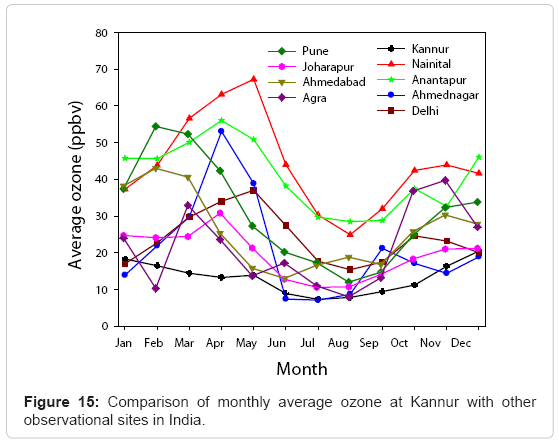
Figure 15: Comparison of monthly average ozone at Kannur with other observational sites in India.
From the Figure 15, it is evident that Nainital, a high altitude site located in the central Himalaya region and in Delhi, the capital city of India recorded the highest O3 mixing ratio during late spring. At Anantapur, Pune, Joharapur and Tranquebar O3 concentrations show distinct maxima in summer season whereas at Dayalbag, Agra and Gadanki it became high during summer/ winter season. At Ahmadabad and Mt. Abu, O3 concentration reaches its peak during autumn/winter and at Trivandrum [66], a tropical coastal site shows a maximum O3 concentration during winter/post monsoon seasons. Among the minimum O3 mixing ratio recorded at these locations, Agra, Gadanki, Dayalbag and Tranquebar register lower concentrations. It is further observed that the O3 minima were found during monsoon and post monsoon seasons at all locations except Gadanki, while the maxima changes with season. Variations of surface O3 concentration recorded at different locations in the Indian subcontinent were mainly due to latitude/longitude variation, population, meteorological parameters, availability of intense solar radiation, differences in the concentrations of precursor gases and anthropogenic activities.
Conclusion
This paper describes the diurnal and seasonal variations of surface O3 and its precursor NOx observed for one year from November 2009 through October 2010 at Kannur University, a rural site lying along the west coast of India. The higher surface O3 concentration observed in the midday and lower concentrations during nighttime was in tune with the solar UV flux. A significant seasonal variation for O3 and NOx mixing ratios at this site was observed. The average O3 mixing ratios were maximum during winter and minimum during the monsoon period. O3 mixing ratio was higher in the winter months at KUC. This may be due to the dominant transport of biogenic VOCs in winter, from the Western Ghats lying east of this site since the air mass movement is from that direction. While in summer, in spite of higher solar flux, O3 concentration was low at this site. This may be due to the cloud cover and the higher abundance of humidity due to proximity with the Arabian Sea. During the southwest monsoon period, O3 concentration was found to be a minimum and it gradually builds up in the post-monsoon season. The seasonal changes in O3 levels are found to be different due to the atmospheric pollution levels. We found good correlations between O3, NO and NO2 which revealed the chemistry of O3 production from NO2 and titration with NO at this location. Further a linear relationship between NO and NOx and NO2 and NOx obtained could be useful in unfolding the chemistry of O3 at this location. The net effect of NOx on O3 concentrations was negative with a decaying exponential correlation indicating a possible VOC sensitive location, which reveals the prominent role of abundant biogenic VOCs on the production of O3 even at lower levels of NO2 present over KUC.
A good correlation between O3, temperature and humidity were obtained which shows that the seasonal variation of O3 has strong dependence on meteorological parameters. This observation further reveals that the marine influence is well defined in this location and other prominent precursors is essential in the O3 chemistry over this location. These observations are useful in understanding the ambient air quality of a location with high population density and the enhanced anthropogenic activities that lead to deterioration in the air quality. The elevated levels of O3 in an industrially less developed area can also affect human health. This will be further ascertained through an analysis of indoor air quality in the area. The results of this study are preliminary and need confirmation with more observation to explore the O3 chemistry and transport with the aid of other gas analyzers like CO, CH4 and VOC.
Acknowledgements
The observations are carried out under the consistent support of ISRO-GBP through AT-CTM program. Authors are grateful to Professor Shyam Lal, Physical Research Laboratory, India for his keen interest in this work. They are grateful to Professor R Ravikrishna, Department of Chemical Engineering, Indian Institute of Technology, Madras, India for analyzing and identifying the organic compounds. Authors thank Dr. Jiye Zeng (NIES, Tsukuba) for providing the METEX model data for calculating air trajectories. One of the authors, (Nishanth T) expresses his gratitude to Indian Space Research Organization for awarding Senior Research Fellowship under ISRO-GBP (ATCTM) programme. Authors wish to thank Editor, Managing Editor of the Journal and the anonymous reviewers for their helpful comments on our manuscript which improve the original scientific contents.
References
- Akimoto H (2003) Global Air Quality and Pollution. Science 302: 1716- 1719.
- Molina LT, Molina MJ (2002) Air Quality in the Mexico Megacity: An integrated Assessment. Kluwer Academic Publishers 96: 141-145.
- Molina MJ, Molina LT (2004) Megacities and Atmospheric Pollution. J Air Manag Assoc 54: 644-680.
- Aneja VP, Schlesinger WH, Erisman JW (2008) Farming pollution. Nature Geoscience 1: 409-411.
- Atkinson R (2000) Atmospheric chemistry of VOCs and NOx. Atmos Environ 34: 2063-2101.
- Han S, Bian H, Feng Y, Liu A, Li X, et al. (2011) Analysis of the relationship between O3, NO and NO2 in Tianjin, China. Aerosol and Air Quality Research 11:128-139.
- Selin NE, Wu S, Nam KM, Reilly JM, Paltsev S, et al. (2009) Global health and economic impacts of future ozone pollution. Environ.Res Lett 4.
- Debaje SB, Kakade AD, Jeyakumar JS (2010) Air pollution effect of O3 on crop yield in rural India. J Hazardous Mat 183: 773–779.
- Avnery S, Mauzerall DL, Liu J, Horowitz LW (2011) Global crop yield reductions due to surface ozone exposure: 1. Year 2000 crop production losses and economic damage. Atmos Environ 45: 2284- 2296.
- Brasseur GP, Kiehl JT, Muller JF, Schneider T, Granier C, et al. (1998) Past and future changes in global tropospheric ozone: impact on radiative forcing. Geophy Res Lett 25: 3807-3810.
- Mickley LJ, Murti PP, Jacob DJ, Logan JA, Koch DM, et al. (1999) Radiative forcing from tropospheric ozone calculated with a unified chemistry climate model. J Geophys Res 104: 30153-30172.
- Chameides W, Walker JCG (1973) A photochemical theory of tropospheric ozone. J Geophys Rese 78: 8751-8760.
- Fishman J, Crutzen PJ (1977) A Numerical Study of Tropospheric Photochemistry Using a One Dimensional Model. J Geophy Res 82: 5897-5906.
- Crutzen PJ, Lawrence MG, Poschl U (1999) On the background photochemistry of tropospheric ozone. Tellus 51: 123-146.
- Crutzen PJ, Heidt LE, Krasnec JP, Pollock WH, Seiler W (1979) Biomass burning as a source of atmospheric gases CO, H2, N2O, NO, CH3Cl and COS. Nature 282: 253-256.
- Chameides WL (1978) The photochemical role of tropospheric nitrogen oxides. Geophs Rese Lett 5: 17-20.
- Ramanathan V, Cicerone RJ, Singh HB, Kiehl JT (1985) Trace Gas Trends and Their Potential Role in Climate Change. J Geophys Res 90: 5547-5566.
- Sillman S, Al-wali KI, Marsik FJ, Nowacki P, Samson PJ, et al. (1995) Photochemistry of ozone formation in Atlanta, GA-Models and measurements. Atmos Environ 29: 3055-3066.
- Sillman S (1999) The relation between ozone, NOx and hydrocarbons in urban and polluted rural environments. Atmos Environ 33: 1821-1845.
- Logan JA, Prather MJ, Wofsy SC, McElroy MB (1981) Tropospheric Chemistry: A Global Perspective. J Geophys Res 86: 7210-7254.
- Kleinman LI, Daum PH, Lee YN, Nunnermacker LJ, Springton SR, et al. (2001) Sensitivity of ozone production rate to ozone precursors. Geophysical Research Letters 28: 2903-2906.
- Kelly NA, Wolff GT, Ferman MA (1984) Sources and sinks of ozone in rural areas. Atmospheric Environment 18: 1251-1266.
- Logan JA (1985) Tropospheric Ozone: Seasonal Behavior, Trend and Anthropogenic Influence. Journal of Geophys Res 90: 10463-10482.
- Cheung VTF, Wang T (2001) Observational study of ozone pollution at a rural site in the Yangtze Delta of China. Atmos Environ 35: 4947-4958.
- Debaje SB, Kakade AD (2006) Measurements of Surface Ozone in Rural Site of India. Aerosol. Air Quality Res 6: 444-465.
- Mioduszewski JR, Yu XY, Morris VR, Berkowitz CM, Flaherty JE (2011) In-Situ Monitoring of Trace Gases in a Non–Urban Environment. Atmos Pollut Rese 2: 89-98.
- Naja M, Lal S (2002) Surface ozone and precursor gases at Gadanki (13.5ºN, 79.2ºE), a tropical rural site in India. J Geophys Res 107: 13.
- Naja M, Chand D, Sahu L, Lal S (2004) Trace gases over marine regions around India. Indian J Marine Sci 33: 95-106.
- Trainer M, Williams EJ, Parrish DD, Buhr MP, Allwine EJ, et al. (1987) Models and observations of the impact of natural hydrocarbons on rural ozone. Nature 329: 705-707.
- Gabusi V, Volta M (2005) Seasonal modelling assessment of ozone sensitivity to precursors in Northern Italy. Atmos Environ 39: 2795-2804.
- Beig G, Gunthe S, Jadhav DB (2007) Simultaneous measurements of ozone and its precursors on a diurnal scale at a semi-urban site in India. J Atmos Chem, 57: 239-253.
- Portmann RW, Solomon S, Fishman J, Olson JR, Kiehl JT, et al. (1997) Radiative forcing of the Earth's climate system due to tropical tropospheric ozone production. J Geophys Res 102: 9409-9417.
- Racherla PN, Adams PJ (2008) The response of surface ozone to climate change over the Eastern United States. Atmos Chem Phys 8: 871-885.
- Lyons WA, Cole HS (1976) Photochemical Oxidant Transport: Mesoscale Lake Breeze and Synoptic-Scale Aspects. J Appl Meteorol 15: 733-743.
- Aneja VP, Das M (1995) Correlation Of Ozone and Meteorology with Hydrogen Peroxide in Urban and Rural Regions of North Carolina. J Appl Meteorol 34: 1890-1898.
- Oltmans SJ, Lefohn AS, Harris JM, Galbally I, Scheel HE, et al. (2006) Long-term changes in tropospheric ozone. Atmos Environ 40: 3156-3173.
- Oltmans SJ (1981) Surface Ozone Measurements in Clean Air. J Geophys Res 86: 1174-1180.
- Volz A, Kley D (1988) Evaluation of the Montsouris series of ozone measurements in the nineteenth century. Nature 332: 240-242.
- Qin Y, Tonnesen GS, Wang Z (2004) One-hour and eight-hour average zone in the California South Coast air quality management district: trends in peak values and sensitivity to precursors. Atmos Environ 38: 2197-2207.
- Alvarez R, Weilenmann M, Favez JY (2008) Evidence of increased mass fraction of NO2 within real-world NOX emissions of modern light vehicles- derived from a reliable online measuring method. Atmos Environ 42: 4699-4707.
- Streets DG, Bond TC, Carmichael GR, Fernandes SD, Fu Q (2003) An inventory of gaseous and primary aerosol emissions in Asia in the year 2000. J Geophys Res 108: 8809-8832.
- Geng F, Tie X, Xu J, Zhou G, Peng L, et al. (2008) Characterizations of ozone, NOx, and VOCs measured in Shanghai, China. Atmos Environ 42: 6873-6883.
- Lee YC, Calori G, Hills P, Carmichael GR (2002) Ozone episodes in urban Hong Kong 1994-1999. Atmos Environ 36: 1957-1968.
- Lu W, Wang X, Wang W, Leung AYT, Yuen K (2002) A preliminary study of ozone trend and its impact on environment in Hong Kong. Environment International 28: 503-512.
- Wang T, Wei XL, Ding AJ, Poon CN, Lam KS, et al. (2009) Increasing surface ozone concentrations in the background atmosphere of Southern China 1994–2007. Atmos Chem Phys 9: 10429-10455.
- Gardner MW, Dorling SR (1999) Neural network modelling and prediction of hourly NOx and NO2 concentrations in urban air in London. Atmos Environ 33: 709-719.
- Corani G (2005) Air quality prediction in Milan: feed-forward neural networks, pruned neural networks and lazy learning. Ecol Model 185: 513-529.
- Juan GS, Jose DMG, Emilio SO, Joan VF, Carrasco JL, et al. (2006) Neural networks for analysing the relevance of input variables in the prediction of tropospheric ozone concentration. Atmos Environ 40: 6173-6180.
- Lu WZ, Wang D (2008) Ground-level ozone prediction by support vector machine approach with a cost-sensitive classification scheme. Sci Total Environ 395: 109-116.
- Ghude SD, Jain SL, Arya BC, Kulkarni PS, Kumar A, et al. (2006) Temporal and spatial variability of surface ozone at Delhi and Antarctica. Inter J Climatol 26: 2227-2242.
- Kumar R, Naja M, Venkataramani S, Wild O (2010) Variations in surface ozone at Nainital: a high-altitude site in the central Himalayas. J Geophys Res 115: 1-12.
- Reddy BSK, Kumar RK, Balakrishnaiah G, Gopal KR, Reddy RR, et al. (2010) Observational studies on the variations in surface ozone concentration at Anantapur in southern India. Atmos Res 98: 125-139.
- Singla V, Satsangi A, Pachauri T, Lakhani A, Kumari KM (2011) Ozone formation and destruction at a sub-urban site in north central region of India. Atmos Res 101: 373-385.
- Mittal ML, Hess PG, Jain SL, Arya BC, Sharma C (2007) Surface ozone in the Indian region. Atmos Environ 41: 6572-6584.
- Khemani LT, Momin GA, Rao PSP, Vijayakumar R, Safai PD (1995) Study of surface ozone behaviour at urban and forested sites in India. Atmos Environ 29: 2021-2024.
- Lal S, Naja M, Subbaraya BH (2000) Seasonal variations in surface ozone and its precursors over an urban site in India. Atmos Environ 34: 2713-2724.
- Nair PR, Chand D, Lal S, Modh KS, Naja M, et al. (2002) Temporal variations in surface ozone at Thumba (8.6ºN, 77ºE)- a tropical coastal site in India. Atmos Environ 36: 603-610.
- Naja M, Lal S, Chand D (2003) Diurnal and seasonal variabilities in surface ozone at a high altitude site Mt Abu (24.6ºN, 72.7ºE, 1680 m asl) in India. Atmos Environ 37: 4205-4215.
- Jain SL, Arya BC, Kumar A, Ghude SD, Kulkarni PS (2005) Observational study of surface ozone at New Delhi, India. Inter J Remote Sens 26: 3515-3524.
- Lal S (2007) Trace gases over the Indian region. Indian J Radio Space Physics 36: 556-570.
- Londhe AL, Jadhav DB, Buchunde PS, Kartha MJ (2008) Surface ozone variability in the urban and nearby rural locations of tropical India. Current Science 95: 1724-1729.
- Ghude SD, Jain SL, Arya BC, Beig G, Ahammed YN, et al. (2008) Ozone in ambient air at a tropical megacity, Delhi: Characteristics, trends and cumulative ozone exposure indices. J Atmos Chem 60: 237-252.
- Reddy RR, Gopal KR, Reddy LSS, Narasimhulu K, Kumar KR, et al. (2008) Measurements of surface ozone at semi-arid site Anantapur (14.62ºN, 77.65ºE, 331 m asl) in India. Journal of Atmos Chem 59: 47-59.
- Renuka S, Satsangi GS, Taneja A (2008) Concentrations of O3, NO2, CO during winter seasons at a semi- arid region- Agra, India. Indian Journal of Radio Space Physics 37: 121-130.
- David LM, Nair PR (2011) Diurnal and seasonal variability of surface ozone and NOx at a tropical coastal site: Association with mesoscale and synoptic meteorological conditions. J Geophy Res 116: D10303.
- Nishanth T, Ojha N, Satheesh Kumar MK, Naja M (2011) Influence of solar eclipse of 15 January 2010 on surface ozone. Atmos. Environ 45: 1752-1758.
- Nishanth T, Praseed KM, Satheesh Kumar MK (2011) Solar eclipse-induced variations in solar flux, j(NO2) and surface ozone at Kannur, India. Meteorology Atmospheric Phys 113: 67-73.
- Nishanth T, Praseed KM, Rathnakaran K, Satheesh Kumar MK, Ravi Krishna R, et al. (2012) Atmospheric pollution in a semi-urban, coastal region in India following festival seasons, Atmos Environ 47: 295-306.
- Winer AM, Peters JW, Smith JP, James N, Pitts Jr (1974) Response of commercial chemiluminescent NO-NO2 analyzers to other nitrogen-containing compounds. Environ Science Technol 8: 1118-1121.
- Finaylson-Pitts BJ, Pitts NJ (1986) Formation of sulfuric and nitric acid in the acid rain and fogs. Atmospheric Chemistry: Fundamentals and experimental Techniques. John Wiley & Sons, New York, USA.
- Steinbacher M, Zellweger C, Schwarzenbach B, Bugmann S, Buchmann B, et al. (2007) Nitrogen oxide measurements at rural sites in Switzerland: Bias of conventional measurement techniques. Geophys Rese Lett 112.
- Warneck P (1988) Chemistry of the natural atmosphere. Academic press, New York, USA.
- Reddy RR, Gopal KR, Narasimhulu K, Reddy LSS, Kumar KR, et al. (2008) Diurnal and seasonal variabilities in surface ozone and its precursor gases at a semi- arid site Anantapur (14.62ºN, 77.65ºE, 331m asl) in India. Inter J Environ Studies 65: 247-265.
- Ahammed YN, Reddy RR, Gopal KR, Narasimhulu K, Basha DB, et al. (2006) Seasonal variation of the surface ozone and its precursor gases during 2001-2003, measured at Anantapur (14.62ºN), a semi-arid site in India. Atmos Res 80: 151-164.
- Seinfeld JH, Pandis SN (2006) Atmospheric Chemistry and Physics: From Air Pollution to Climate Change. John Wiley & Sons Publications, New York, USA.
- Song F, Shin JY, Atresino RJ, Gao Y (2011) Relationships among the springtime ground-level NOx, O3 and NO3 in the vicinity of highways in the US East coast. Atmos Pollut Res 2: 374-383.
- Dalsøren SB, Eide MS, Endresen Ø, Mjelde A, Gravir G, et al. (2008) Update on emissions and environmental impacts from the international fleet of ships. The contribution from major ship types and ports. Atmos Chem Phys 8: 18323-18384.
- de Gouw JA, Middlebrook AM, Warneke C, Ahmadov R, Atlas EL, et al. (2011) Organic Aerosol formation downwind from the deepwater horizon oil spill. Science 331: 1295-1299.
- Porg (1997) Ozone in the United Kingdom. Fourth Report of the UK Photochemical Oxidants Review Group, Department of the Environment, Transport and the Regions, London. Published by the Institute of Terrestrial Ecology, Bush Estate, Penicuik, Midlothian, EH26 0QB, UK.
- Jacob DJ, Heikes EG, Fan SM, Logan JA, Mauzerall DL, et al. (1996) Origin of ozone and NOx in the tropical troposphere: A photochemical analysis of aircraft observations over the South Atlantic basin. J Geophys Res 101: 24235- 24250.
- Wood EC, Bertram TH, Wooldridge PJ, Cohen RC (2005) Measurements of N2O5, NO2, and O3 east of the San Francisco Bay. Atmos Chem Phys 5: 483-491.
- Brown SS, Neuman JA, Ryerson TB, Trainer M, Dube WP, et al. (2006) Nocturnal odd-oxygen budget and its implications for ozone loss in the lower troposphere. Geophy Res Lett 33.
- Derwent RG, Middleton DR, Field RA, Goldstone ME, Lester JN, et al. (1995) Analysis and interpretation of air quality data from an urban roadside location in central London over period from July 1991 to July 1992. Atmos Environ 29: 923-946.
- Clapp LJ, Jenkin ME (2001) Analysis of the relationship between ambient levels of O3, NO2 and NO as a function of NOx in UK. Atmos. Environ 35: 6391-6405.
- Kourtidis KA, Ziomas I, Zerefos C, Kosmidis E, Symeonidis P, et al. (2002) Benzene, toluene, ozone, NO2 and SO2 measurements in an urban street canyon in Thessaloniki, Greece. Atmos Environ 36: 5355-5364.
- Palacios M, Kirchner F, Martilli A, Clappier A, Martin F (2002) Summer ozone episodes in the Greater Madrid area. Analyzing the ozone response to abatement strategies by modeling. Atmos Environ 36: 5323-5333.
- Saiz-Lopez A, Notario A, MartÃnez E, Albaladejo J (2006) Seasonal evolution of levels of gaseous pollutants in an urban area (Ciudad Real) in central-southern Spain: a DOAS study. Water Air and Soil Pollution 171: 153-167.
- Saiz-Lopez A, Adame JA, Notario A, Poblete J, BolÃvar JP, et al. (2009) Year round observations of NO, NO2, O3, SO2 and toluene. Water Air and Soil Pollution 200: 277-288.
- Notario A, Bravo I, Adame JA, D´iazde MY, Aranda A, et al. (2011) Analysis of NO, NO2, NOx, O3 and oxidant (OX = O3 + NO2) levels measured in a metropolitan area in the southwest of Iberian Peninsula. Atmos Res 104: 217-226.
- Wayne RP (2002) Chemistry of Atmospheres, ed. Oxford University Press. 3rd Edition.
- Nishanth T, Satheesh Kumar MK, Valsaraj KT (2012) Variations in surface ozone and NOx at Kannur: A tropical, coastal site in India. J Atmospheric Chemistry. DOI: 10.1007/s10874-012-9234-5
- Zeng J, Tohjima Y, Fujinuma Y, Mukai H, Katsumoto M (2003) A study of trajectory quality using methane measurements from Hateruma Isaland. Atmos Environ 37: 1911-1919.
Citation: Nishanth T, Praseed KM, Satheesh Kumar MK, Valsaraj KT (2012) Analysis of Ground Level O3 and Nox Measured at Kannur, India. J Earth Sci Climate Change 3: 111. DOI: 10.4172/2157-7617.1000111
Copyright: ©2012 Nishanth T, et al. This is an open-access article distributed under the terms of the Creative Commons Attribution License, which permits unrestricted use, distribution, and reproduction in any medium, provided the original author and source are credited.
Select your language of interest to view the total content in your interested language
Share This Article
Recommended Journals
Open Access Journals
Article Tools
Article Usage
- Total views: 18379
- [From(publication date): 6-2012 - Dec 21, 2025]
- Breakdown by view type
- HTML page views: 13376
- PDF downloads: 5003