Research Article Open Access
A Machine Learning Approach for Light-Duty Vehicle Idling Emission Estimation Based on Real Driving and Environmental Information
Qing Li1*, Fengxiang Qiao1and Lei Yu21Innovative Transportation Research Institute, Texas Southern University, 3100 Cleburne Street, Houston, 77004, Texas, USA
2College of Science, Engineering and Technology, Texas Southern University, Texas, USA
- *Corresponding Author:
- Qing Li
Innovative Transportation Research Institute
Texas Southern University, 3100 Cleburne Street
Houston, 77004, Texas, USA
Tel: 713-313-7532
E-mail: liq@tsu.edu
Received date: December 07, 2016; Accepted date: December 15, 2016; Published date: December 22, 2016
Citation: Li Q, Qiao F, Yu L (2016) A Machine Learning Approach for Light-Duty Vehicle Idling Emission Estimation Based on Real Driving and Environmental Information. Environ Pollut Climate Change 1:106.
Copyright: © 2016 Li Q, et al. This is an open-access article distributed under the terms of the Creative Commons Attribution License, which permits unrestricted use, distribution, and reproduction in any medium, provided the original author and source are credited.
Visit for more related articles at Environment Pollution and Climate Change
Abstract
The conventional models for idling emission estimation are mainly based on ambient temperature and the status of vehicle itself, such as vehicle type/size, age and accumulated mileage and fuel type. Instant vehicle activity information is seldom taken into account. In this research, a machine learning approach is proposed to dynamically estimate vehicle emission rates while idling, based on real-world driving tests on more than 1,600 km highways in the State of Texas in the USA. One driver drove a dedicated light-duty gasoline vehicle on various types of roads, including interstate freeways, farm roads, state highways, and arterial road. During each episode of idling, rates of vehicle exhaust emissions, including carbon dioxide (CO2), carbon monoxide (CO), hydrocarbon (HC) and nitrogen oxides (NOx) were measured by a Portable Emission Measurement System (PEMS). Meanwhile, the real-time vehicle engine information of the test vehicle, such as revolutions per min, intake air temperature, and environmental information (e.g. ambient temperature), were collected through the On-board Diagnosis II port. Five machine learning algorithms were applied to build up idling emission models to illustrate the nature of emission patterns. Results show that Boosted and Bagged Decision Trees (BBDT) based idling emission model was identified as the best-fit ones for dynamic idling emissions with better prediction performance.
Keywords
Vehicle emission; Idling emission; Machine learning algorithm; Decision trees; KNN model; Field test.
Introduction
Idling refers to the vehicle operation, when a vehicle’s engine is running, but not in motion [1,2]. Though usually individual idling episode is very small in a driving trip, the cumulative impacts of idling are enormous. In the United States, more than 6 billion gallons of fuel yearly were spent on the avoidable idling operations [3], leading to a total of 5, 988.66 billion ton of carbon dioxide (CO2) emissions. What’s more, the gigantic byproducts of nitrogen oxides (NOx), carbon monoxide (CO), and hydrocarbon (HC) are toxic to environment and humans [4]. An insight into the idling emission pattern is essential to prevent the unnecessary toxic exhaust from emitting.
The idling can be discretionary or non-discretionary. Discretionary idling occurs only when the driver chooses to stop and idle, while non-discretionary idling takes place during normal driving due to the restrictions of traffic signals, signs and congestions [5]. The nondiscretionary idling lasts normally shorter under a hot start [6], which is often operated during congestion. Many strategies have been implemented to release congestion related non-discretionary idling emissions, such as optimized signal control and eco-driving [7] and improved configuration of drive-through facilities [8]. Though many previous studies have been conducted to explore the idling emission patterns [9,10], most of them usually focus on the emission impacts of a vehicle itself, such as vehicle type/size, age and accumulated mileage, fuel type, and vehicle maintenance conditions, and ambient temperature [11]. The exhaust emissions are mostly statically monitored. In fact, most idling modes are followed with a series of vehicle operations, which transition could result in different engine activities, such as revolutions per min (rpm), intake air temperature (IAT), manifold absolute pressure (MAP), from those monitored during the lab idling tests.
Besides, idling emission estimation is usually embedded into the exhaust emissions attributed by other vehicle operations, such as acceleration and braking, during modeling. The most common used model is the Motor Vehicle Emission simulator (MOVES), which is developed by Environmental Protection Agency (EPA). Other emission models include the Emission Factors (EMFAC) model developed by California Air Resources Board (CARB), the international vehicle Emission (IVE) model in most developing countries, and the Computer Program to calculate Emissions from Road Transport (COPERT) model developed by European Commission Environmental Protection Agency [2]. These macroscopic models statistically use some types of microscopic emission information based on standard emission measurement. For example, MOVES estimates idling emissions by emission rates that are obtained by drive cycles [2,11]. No doubt that these emission rates can simplify the exhaust emission estimation at a regional scale. However, such estimates fail to demonstrate the exhaust emission patterns during an idling mode. Besides, the statistical models are based on a number of assumptions or often end up over fitting.
Comparably, the recently developed machine learning techniques, such as K-Nearest Neighbor (KNN) model, Neural Network, Boosted and Bagged Decision Trees (BBDT), can possibly provide more reliable, repeatable decisions and results. The machine learning techniques learn from measured computations without rules-based programming and conducts prediction on the fly. The most advantage is that there is no any continuity of boundary in the machine learning algorithm and the distribution of dependent or independent variables do not need to be specified [12]. This research attempts to identify a machine learning algorithm for training a best-fit idling emission model, based on field driving tests and real-time environmental information. The best-fit model can illustrate the nature of exhaust emission patterns during idling, and provides reliable and highly accurate estimation results.
Methodology
Machine learning algorithms
Five machine learning algorithms were applied to build idling emission models, including KNN, Neural Network, BBDT, CHAID and Support Vector Machine (SVM) and were screened by comparing their relative errors. The relative error is the ratio of the sum of squared errors for the dependent variable to the sum of squared errors for the null model. A smaller relative error indicates a higher accuracy of prediction. The first two built-up models with lower relative errors were further analyzed, in terms of Root Mean Square Error (RMSE) and the correlation coefficients (R) of the fitted regression lines for each emission index. The better-fit model was identified by a lower relative error, a lower RMSE, and a higher absolute R.
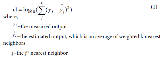
KNN model: As an instance-based learning (i.e., lazy learning), the KNN algorithm is one of the simplest machine learning algorithms. KNN is a model that predicts the value of an output variable based on the values of its nearest neighbors [13]. More specifically, it is a method to recognize the pattern of data without requiring an exact match to any stored patterns or cases. By this mode, similar cases are closely gathered to each other. The distance between cases is the measure of similarity. There will be many neighbors for each case. The best number of neighbors is called k and specified by a crossed check for error log (el) presented in Equation (1).
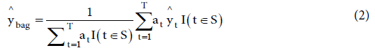
BBDT model: BBDT model is a result of regression trees or classification trees and bagging, which is an ensemble learning method. Multiple decision trees are generated and bagged into an ensemble. For the idling emission estimations, individual tree grows deeply, based on regression trees. The bagging is a training process of resampled data. For each resampling, the unique observations are divided into two groups: bootstrap samples for training and out of bag samples for validation. The predictive power of the trained ensemble is indicated by the average errors from the out-of-bag samples. The prediction algorithm is expressed as Equation (2) [14].
where:
 =the prediction from tree t in the ensemble
S=the set of indices of selected trees that comprise the prediction
at=the weight of tree t
I (t∈S) =1 if t is the set S, otherwise 0
Neural network: The artificial Neural Networks are based on simple mathematical models of the brain. The Levenberg-Marquardt algorithm is one of the typical methods to train the networks (structure, weights and bias) using the multilayer perception procedure [15,16]. The training process stops automatically when generalization no longer improve, indicating by an increase in the mean square error of the validation samples. In this research, a structure of 1 hidden layer and 10 neurons was determined.
SVM model: SVM models are supervised learning models, the algorithms of which analyze data for classification and regression [17]. In the idling emission case, SVM maps emission data to a highdimensional feature space for classification, regardless of whether the data are linearly separable. Once the boundary between categories is found, the data are transformed by the mathematical function of kernel. After the transformation, the boundary can be defined by a hyperplane. The response of new data can be predicted by classifying them into categories based on their features [18].
CHAID model: CHAID stands for CHi-squared Automatic Interaction Detection, and is a type of decision tree technique, which can be used for prediction as well as classification [19]. The optimal splits are identified by significance testing of chi-square independence. The CHAID algorithm consists of three steps: merging the pairs of categories showing the least significant difference, splitting for deep growing, and stopping when all categories differ at the specified testing level. A tree keeps growing by repeating these three steps at each node starting from the root node [20].
Accuracy estimation of predicted responses
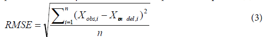
The accuracies of the five machine learning based idling emission models are compared by Root-Mean-Square Error (RMSE) and Pearson product-moment correlation coefficient R. The RMSE is commonly used as a measure of the difference between observed values and predicted values by a model, which is expressed in Equation (3).
Where,
Xobs, i=the ith observed value
Xmodel, i=the modeled value at the ith data prediction
On the other hand, the fitting level of the predicted values to the observed values is measured by the R value, which is obtained by Equation (4)
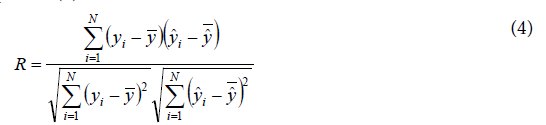
The idling emission model that is able to provide predicted responses with the lowest RMSE and the absolutely higher R value is identified as the best-fit model.
Test plan and data collection
The non-discretionary idling emission pattern is addressed in this study, which is produced by temporal idles for traffic signals and congestion blockages. The vehicle engine in this case can be regarded as already being hot for sufficiently longer time. The structure and parameters of the model would be calibrated from input-output data pairs, which were obtained from on-road driving tests.
Figure 1a illustrates the dedicated light-duty test vehicle, which is a 2004 Subaru Forester with four cylinders and 2.5 liters displacement, auto transmission. Its vehicle weight was 3,100 lb; the test weight was 3,500 lb, with 165 horse power at 5,699 rpm and a torque of 225 Nm at 4,000 rpm. The fuel type is gas and the mileage at start of test was 16,496 km (10,250 miles). Figure 1b is the PEMS placed on the back seat of the test vehicle. A plastic tube from the PEMS is connected to the tailpipe of the vehicle to suck in continuous exhaust emissions for measurement. A global positioning system (GPS) was placed on top of the vehicle to record the instant geolocation information. The sampling rate of the PEMS as well as GPS is 1 Hz (once per sec).
The test vehicle was employed to drive through approximately 1,600 km highways with different types of roads in the State of Texas, USA, including interstate freeways, farm roads, state highways, and arterial roads. The specific idling measurements on each highway are listed in Table 1.
Table 1 shows that a total of P34H14M01S (i.e., a period of 34 h 14 min and 1 s) driving duration on these highways, while the total 221 episodes of idles lasted for P02H23M56S with an average of 39.07 s for each idle. The test sites cover a geologically wider range in the State of Texas.
The vehicle activity and engine information were recorded by connecting the PEMS with an on-board diagnostic (OBD) II port of the test vehicle, during each idling period for congestion or traffic controls, such as traffic signals or stop signs. The collected information combined with each idling duration serves as input variables, including revolutions per min (rpm), Intake Air Temperature (IAT), Manifold Absolute Pressure (MAP), Ambient Air Temperature (AAT), and Idling Duration (ID). Meanwhile, the PEMS was used to measure real-time exhaust emission rates, including CO, CO2, NOx and HC, which are the output variables of modeling.
Figure 2 shows a screenshot of the PEMS records at a sampling frequency of 1 Hz. Column A is the recording time, columns B-E are part of the OBD II information that were flew into the PEMS, column F indicates the source gas analyzer used to measure emissions (from gas analyzer 1 or 2 or both), columns G to K are measured emissions and fuel consumption, column L is the Coordinated Universal Time (UTC), columns O-Q are GPS information, and column R is the realtime driving speed from OBD II.
The total input-output data pairs were divided into three parts for training, validation, and testing. Seventy percent of data pairs were trained by the five algorithms. During the training process, the classification, network and regression, are adjusted according to its errors. Another 15% of the data pairs were used to measure generalization as validation samples and to halt training when the generalization stops improving. The last 15% of the data pairs serves as testing samples, which do not have effect on training and provide an independent measure of modeling performance during and after training.
Results and Discussion
Comparison of relative errors among models
A total of 8,637 data pairs were collected during the idling modes in the real driving tests, which were all recorded at hot engine status. Five machine learning based idling emission models were developed. The relative errors for each emission index are listed in Table 2.

Figure 1: a) The test vehicle b) PEMS placed inside the test vehicle.
| City | Highway | Date | Number of Idling | Total Test Hours | Total Idle Duration |
|---|---|---|---|---|---|
| Austin | TX-183 (between Loop 1 and 45) | 09/24/2015 | 21 | P04H04M50S | P03M41S |
| El Paso | Alameda Ave. | 04/15/2015 | 33 | P06H43M25S | P32M13S |
| El Paso | I-10 | 04/16/2015 | 38 | P03H00M52S | P03M40S |
| Angleton | FM 523 | 06/11/2015 | 18 | P07H22M00S | P18M18S |
| League City | I-45 | 06/12/2015 | 51 | P02H28M37S | P08M51S |
| Magnolia | FM1486 | 01/27/2015 | 22 | P04H32M35S | P37M05S |
| Arcola | FM521 | 06/05/2015 | 18 | P02H38M25S | P29M49S |
| Hitchcock | I-45 | 06/10/2015 | 20 | P03H23M17S | P10M19S |
| Total | 221 | P34H14M01S | P02H23M56S | ||
Table 1: The description of test sites.

Figure 2: Screenshot of the recorded data from PEMS for a test.
In Table 2, the relative errors of the four emission indexes by KNN are relatively closer to the ones by BBDT, ranged from 1% (for CO2 by BBDT) to 15% (for CO by KNN). These two algorithms perform apparently smaller relative errors than Neural Network, CHAID and SVM models. Thus, the KNN and BBDT based idling emission models were selected for further analyses in the next section.
Besides, it is worth noting that except the CHAID algorithm, other four algorithms are able to predict the CO2 emissions with smaller errors, whereas the five algorithms also provide CO and NOx estimations with comparably higher relative errors. This implies that the emission patterns of CO and NOx could be different from CO2 and HC.
KNN modeling results
Figure 3 illustrates the fitted regression lines between the observed and estimated emissions by KNN models from the validation tests. The greater absolute value of R indicates higher correlation between the estimated emissions and the observed emissions. Figures 3a and 3c shows that the estimated CO2 and HC emissions are highly correlated to their corresponding observed values with the R value of 0.94 and 0.85, respectively. The R of 0.58 for NOx could be constrainedly considered as correlated relationship between the estimated and observed values, whereas the R of 0.33 for the CO tells that their relationship is relatively week. Similar fitting results are shown in Figure 4 for the testing phase, in which the correlation coefficients for the CO, HC and NOx , decline slightly to 0.17, 0.78 and 0.53, respectively.
BBDT modeling results
Figure 5 shows the fitted regressions lines between the observed and estimated emission rates by the BBDT algorithm in the validation tests. Like the KNN based emission models, the estimated CO2 and HC emission values by the BBDT highly correlate to the corresponding observed emission values with the R value of 0.98 and 0.91, respectively. Furthermore, the CO and NOx estimations by the BBDT algorithm perform overall higher correlation relationship with the observed values than by the KNN algorithm for the R values of 0.49 and 0.52, respectively.
| Algorithm | CO2 | CO | HC | NOx |
|---|---|---|---|---|
| KNN | 2% | 15% | 5% | 11% |
| BBDT | 1% | 10% | 3% | 8% |
| Neural Network | 3% | 23% | 7% | 16% |
| CHAID | 50% | 75% | 17% | 73% |
| SVM | 2% | 67% | 33% | 99% |
Table 2: The relative errors of the five machine learning based idling emission models.
| Algorithm | Phase | CO2 (g/s) | CO (mg/s) | HC (mg/s) | NOx (mg/s) |
|---|---|---|---|---|---|
| KNN | Validation | 0.19 | 7.47 | 0.29 | 1.95 |
| Testing | 0.21 | 9.73 | 0.35 | 2.24 | |
| BBDT | Validation | 0.10 | 6.46 | 0.22 | 1.82 |
| Testing | 0.08 | 6.24 | 0.19 | 2.56 |
Table 3: RMSE of validation and testing results by KNN and BBDT based idling emission models.
In the testing phase shown in Figure 6, though there is a subtle decrease in R for the NOx emissions with 0.44, the R value for the CO contrarily increase to 0.59. As a whole, the exhaust emission values estimated by the BBDT algorithm are more correlative to the observed emission values than the estimated emission values by the KNN algorithm.
Comparison of RMSE between KNN and BBDT based models
Table 3 depicts the RMSEs of the validation and testing results for the four emission indexes. General speaking, there are subtle differences in the RMSEs between the validation and testing results by the KNN and BBDT algorithms, respectively, which means the two built-up idling emission models are able to provide reliable estimated results.

Figure 3: Fitted regression lines for validation phase by KNN idling emission model.

Figure 4:Fitted regression for testing phase by KNN based idling emission model.

Figure 5:Fitted regression for validation phase by BBDT based idling emission model.

Figure 6:Fitted regression for testing phase by BBDT based idling emission model.
| Model | CO2 | CO | HC | NOx | |
|---|---|---|---|---|---|
| PEMS | Observed | 1.283 | 1.659E-03 | 3.732E-04 | 4.660E-04 |
| BBDT | Estimated | 1.282 | 1.864E-03 | 3.672E-04 | 4.433E-04 |
| MOVES | Estimated | N/A | 1.978E-02 | 7.453E-04 | 9.764E-04 |
Table 4: Comparison of average emission rates (g/s).
Compared with the RMSEs by the two algorithms for each emission index at the two phases, the RMSEs by the KNN algorithm for the CO2, CO, and HC emissions are slightly greater than those by the BBDT algorithm. The NOx emission estimations by the two algorithms are similar to each other. This implies that the BBDT based idling emission model performs better prediction performance. Therefore, the BBDT emission model was identified as the best-fit models among the five developed machine learning emission models for its lower relative errors, higher absolute R values, and lower RMSEs. Besides, the average idling emission rates estimated by the best-fit model, the BBDT based emission model, were compared with the observed values measured by PEMS and the estimated values by MOVES for a light-duty gasoline vehicle. Table 4 shows the comparison results.
Note: N/A=the emission rate is not available from source [11]
In Table 4, the MOVES estimated values were the average emissions of all light-duty vehicles. It is obvious that, the BBDT estimated emission rates are very close to the observed ones, whereas both the observed and the estimated emission rates are quite different from the MOVES estimations for average light-duty vehicles. In other words, the built-up BBDT based idling emission model presents better predictive power for this specific test vehicle.
Conclusion
Field vehicle idling emission tests were conducted in several different cities in the State of Texas. Vehicle activity information, engine information, and real-time exhaust emissions during each idling period were recorded and analyzed to characterize the pattern for modeling. A total of five machine learning based idling emission models were developed. Among the five models, the BBDT and KKN based idling emission models presented better predictions with lower relative errors, ranged from 1% for CO2 to 15% for CO. The prediction performance of the two models was compared by their RMSEs for each emission index. The RMSEs by the BBDT based idling emission model for the CO2, CO and HC exhaust emissions at the validation phase as well testing phase, were overall smaller than those by the KKN based emission models. Therefore, the BBDT based idling emission model was identified as the best-fit model. Besides, the estimated emission rates by the best-fit model were very close to the observed emission rates by PEMS.
The BBDT built-up model can accurately and dynamically estimate vehicle idling emissions. Such a model can be easily embedded into a smartphone or tablet via a suitably developed application, so as to promptly display vehicle idle emissions while being halted at red lights or in a queue of congestions.
Acknowledgement
The authors acknowledge that this research is supported in part by the National Science Foundation (NSF) under grants #1137732. The opinions, findings, and conclusions or recommendations expressed in this material are those of the author(s) and do not necessarily reflect the views of the funding agencies.
References
- Qiao F, Yu L, Soltani V (2006) Characteristics of truck idling emissions under real-world conditions. TRB 85th Annual Meeting Compendium of Papers CD-ROM. Washington DC, United States.
- Farzaneh M, Zietsman J, Lee DW, Johnson J, Wood N, et al. (2014) Texas-Specific drive cycles and idle emissions rates for using with EPA'S moves model-final report.
- Energy Systems (2016) Reducing vehicle idling.
- Li Q, Qiao F, Yu L (2016) Vehicle emission implications of drivers smart advisory system for traffic operations in work zones. J Air Waste Manag 66: 446-455
- Zietsman J, Perkinson DG (2003) Heavy-duty diesel vehicle (HDDV) idling activity and emissions study: Phase 1 - Study design and estimation of magnitude of the problem. Texas Commission on Environmental Quality, Austin, Texas.
- Qiao F, Yu L, Li L (2007) Estimating impact of nonrecurring congestion on vehicle emissions. TRB 86th Annual Meeting Compendium of Papers CD-ROM. Washington DC, United States.
- Tang P, Azimi M, Qiao F, Yu L (2016) Examining the impact of eco-driving advising strategies on vehicle emissions for vehicles traveling within intersection vicinities. TRB 95th Annual Meeting Compendium of Papers CD-ROM. Washington DC, United States.
- Hill K, Qiao F, Azimi M, Yu L (2014) Impacts of restaurant drive-through configurations on vehicle emissions. TRB 93rd Annual Meeting Compendium of Papers CD-ROM. Washington DC, United States.
- Lim H (2003) Study of exhaust emissions from idling heavy duty diesel trucks and commercially available idle reducing devices. SAE Technical Paper.
- Ashrafur Rahman SM, Masjuki HH, Kalam MA, Abedin MJ, Sanjid A, et al. (2013) Impact of idling on fuel consumption and exhaust emissions and available idle-reduction technologies for diesel vehicles- A review. Energ Convers Manage 74: 171-182.
- Environmental Protection Agency (EPA) (2008) Idling vehicle emissions for passenger cars, light-duty trucks and heavy-duty trucks. Office of Transportation and Air Quality.
- Srivastava T (2015) Difference between machine learning and statistical modeling.
- Altman NS (1992) An introduction to kernel and nearest-neighbor nonparametric regression. Am Stat 46: 175-185.
- Meinshausen N (2006) Quantile regression forests. J Mach Learn Res 7: 983–999.
- Marquardt DW (1963) An algorithm for least-squares estimation of nonlinear parameters. Journal of the Society for Industrial and Applied Mathematics 11: 431-441.
- Li Q, Qiao F, Yu L (2016). Neural network modeling of in-vehicle noises with different roadway roughness. Proceedings of the 11th Asia Pacific Transportation Development Conference and 29th ICTPA Annual Conference - Bridging the East and West: Theories and Practices of Transportation in the Asia Pacific. May 27-29, 2016. Hsinchu, Taiwan. Paper
- Cortes C, Vapnik V (1995) Support-vector networks. Machine Learning 20: 273.
- Press WH, Teukolsky SA, Vetterling WT, Flannery BP (2007) Section 16.5. Support Vector Machines. Numerical Recipes: The Art of Scientific Computing (3rd ed.). New York: Cambridge University Press. ISBN 978-0-521-88068-8.
- Section 16.5. Support Vector Machines
- Kass GV (1980) An exploratory technique for investigating large quantities of categorical data. Applied Statistics 29: 119-127.
Relevant Topics
Recommended Journals
Article Tools
Article Usage
- Total views: 6892
- [From(publication date):
January-2017 - Aug 24, 2025] - Breakdown by view type
- HTML page views : 5839
- PDF downloads : 1053