Analysis of Temperature Trends in Sutluj River Basin, India
Received: 14-Jul-2014 / Accepted Date: 24-Sep-2014 / Published Date: 30-Sep-2014 DOI: 10.4172/2157-7617.1000222
Abstract
Surface air temperature is an important climatic variable that drives the hydrological cycle. Precipitation and runoff production are impacted by surface air temperature changes and are, therefore, important for water resources planning, irrigation and agriculture. Focusing on the Sutlej Basin in the Himalayan region, the present research is aimed at utilizing observational evidence to evaluate the response of the region to global warming through investigation of temperature trends. Trends in long-term average annual and seasonal surface air temperature, and several temperature indices at eight stations in the Sutlej River basin have been examined using Mann-Kendall non-parametric test. Six stations exhibited increasing trends in annual average maximum temperature with two being statistically significant. The trends in annual average minimum temperature were mixed; three of eight stations exhibited statistically significant decreasing trends. Some higher elevation stations exhibited clear warming trends both in maximum and minimum temperatures. Analysis of seasonal temperature data indicated that the warming was more pronounced in winter and spring than in summer and autumn. Trends in temperature indices considered in this paper were predominantly increasing. The predominant pattern of increased warming in the basin could have implications for water availability as the snow and glacier melt contribution to annual runoff at Bhakra reservoir is estimated at 59%. The analysis shows that even within a small area, there is variability in the magnitude and direction of historic temperature trends. Some of these variations could be partially attributed to data reliability.
Keywords: Climate; Mann kendall; Satluj; Temperature; Trends
6504Introduction
Evidence from climate models suggests that the global climate is changing in an unprecedented manner, mainly due to rapid increase in the atmospheric concentration of greenhouse gases. The increase in greenhouse gas emissions in most parts of the world, including India is likely to continue in the near term. The Fourth Assessment Report (AR4) of the Intergovernmental Panel on Climate Change [1] indicates a global warming of about 0.2°C per decade for a range of emission scenarios described in the Special Report on Emissions Scenarios (SRES) over the next two decades. Even if the concentrations of greenhouse gases and aerosols were to stabilize at year 2000 levels, a 0.1°C per decade increase in global temperatures is projected [2]. The Intergovernmental Panel on Climate Change (IPCC) report [1] clearly indicates the likelihood of considerable warming over sub regions of South Asia, with greater warming in winter than in summer. Results of multimodal Global Climate Model (GCM) run under B1 and A1F1 scenarios project an increase in average surface air temperature over South Asia, with the greatest increase being projected for winter months [3]. The projected rise in temperature for winter months exceeds the global mean surface temperature rise (1.8 to 4°C) at 2090-2099 relative to 1980-1999 under B1 and A1F1 scenarios [2]. Results of GCMs suggest that absorbing aerosols have significantly influenced warming of the lower troposphere over Asia [4]. The Himalayan region, which provides a critical source of water for China, India and Pakistan, is among the areas most vulnerable to global warming. Over the last century, global mean temperatures increased at a rate of 0.07°C per decade, but the warming has not been globally uniform, with high northern latitudes particularly affected [5]. A recent study by Ohmura [6] based on observations from the last 50 to 125 years found enhanced warming with elevation in about two-thirds of the mountain regions examined.
Surface air temperature is an important variable that impacts the dynamics of atmospheric processes. The vigor of the hydrological cycle is intensified by the increase in air temperature caused by increasing levels of CO2 in the atmosphere [7]. Due to increased concentration of greenhouse gases and aerosols in the atmosphere, perceptible changes in temperature patterns are likely. Since precipitation and runoff production are significantly impacted by temperature changes such changes are considered important for water resources planning, irrigation and agricultural production. In addition, hydrological systems are anticipated to experience, not only changes in average availability of water, but also changes in extremes [8,9]. However, the impacts of climate change on hydrological systems may vary from region to region. India is especially vulnerable to the impacts of climate change mainly due to rapid industrialization, population pressures, and high rate of economic development in the country. In an economy where about half of the people depend upon agriculture and allied activities for their livelihood, the significance of climate change cannot be overstressed.
Several studies have reported warming in the South Asian region including India. Hingane et al. [10] found a warming of about 0.4°C in India during the last eight decades, largely due to rise in maximum temperatures. Rao [11] presented long-term changes of annual and seasonal surface air temperatures and precipitation of the Mahanadi river basin in India, for the period 1901-1980. A significant warming trend was detected in the average maximum, average minimum and average mean temperatures of the basin. Sinha et al. [12] reported that changes in annual temperatures may be attributed partly to the rise in the minimum temperature caused by intensive urbanization. Analysis of mean annual temperatures by Pant and Kumar [13] revealed an increase of 0.57°C per 100 years. Arora et al. [14] conducted an analysis of temperature trends over India using Mann-Kendall test, and linear regression method. The post monsoon season showed an increase of 0.94°C per 100 years, whereas the winter season showed an increase of 1.1°C per 100 years. Singh et al. [15] carried out an extensive analysis of basin-wide temperature trends in central and northeast India. A warming trend was found in seven, and a cooling trend in two river basins. Cheema et al. [16] analyzed monthly means of 60 year records of temperature of the city of Faisalabad and found that the summer season is becoming cooler whereas the winter is becoming warmer.
Climate change concerns in the Himalayan region are diverse and range from floods, droughts, landslides [17], human health, biodiversity, endangered species, agriculture livelihood, and food security [18]. The region has the largest snow and ice cover in the world outside the polar region, and is, therefore, known as the third pole [19]. The Ganges, the Brahmaputra and the Indus constitute the three major river systems in the region, and are fed by glaciers and seasonally renewed snow in the Himalayas. A study by the Government of India [20] showed that the Himalayan states account for more than 70% of India’s hydropower potential in terms of installed capacity greater than 25 MW. The waters of the Himalayan region play an important role in the agriculture, hydropower, and tourism thus impacting the Indian economy in a significant manner. The fragile landscape of the Himalayan region makes it highly vulnerable to the current and future climate change impacts in the region [21]. With more than 1000 glaciers in the region, the vulnerability of the region to the rising temperatures cannot be overstressed. While hydropower is impacted both by temperature and precipitation, a study by Rathore et al. [22] has suggested that the 1°C rise in temperature by 2040 alone could reduce the hydropower generation mainly due to the reduction in runoff by 8-20% depending upon the season. The authors claim that the reduced runoff is likely due to the reduction in snow and glacier extent by 2040. Studies of surface air temperatures in the Himalayan region are, however, few. Shrestha et al. [23] analyzed maximum surface air temperature data from 49 stations in Nepal for the period 1971–94 revealing warming trend after 1977 ranging from 0.06 to 0.12°C per year in most of the Middle Mountain and Himalayan regions, whereas the Siwalik and Terai regions showed warming trends of less than 0.03°C per year. Cook et al. [24] found that 20th century surface air temperatures over Kathmandu have been cooling in general during the pre-monsoon (February–May) and monsoon (June–September) seasons. Only during the post-monsoon (October–January) season is there some suggestion of warming, mainly since 1960. These results are in contrast to some of the conclusions of Shrestha et al. [25] which suggested a more general warming trend in Nepal since the mid-1970s.
Fowler and Archer [26] examined seasonal and annual temperature trends at several climate stations in the Hindu Kush and Karakoram mountains of the Upper Indus Basin. A significant increase was observed in mean and maximum winter temperatures while mean and minimum summer temperatures showed consistent decline. Fowler and Archer [26] found a consistent increase in Diurnal Temperature Range (DTR) in all seasons and annual dataset, which is in direct contrast to studies in most parts of the world that show a narrowing of DTR [27,28]. Khattak et al. [3] investigated trends in several hydro-meteorological variables in the Indus River basin. Dash et al. [29] report that, during the last few decades, the Tibetan Plateau and the Himalayan region have been warming at a rate higher than that in the last century. An increase of 0.5°C in annual average maximum temperature during 1971-2005 was reported compared to 1901-1960 period. Dimri and Dash [30] reported a warming trend over western Indian Himalayas, with the greatest increase in TMX ranging from 1.1 C to 2.5°C. Immerzeel [31] found a basin wide warming trend of 0.6°C/ 100 year for the 1901-2002 gridded dataset for the part of the Brahmaputra basin that lies in the eastern Indian Himalaya and Tibetan Plateau.
The analysis of hydro-meteorological data for trends is often required for conducting a detailed assessment of climate change impacts and climate variability on the water resources of mountainous catchments [32]. The contribution of snow and glacier melt to streamflow at Bhakra, the major reservoir in the Satluj basin, is around 59% [33]. There have been increases in temperatures worldwide, and several climate models suggest that this trend will continue under climate change. There is some debate whether the warming will be enhanced at high elevations, such as in the Himalayan region. Any discernible trends in surface air temperature are likely to adversely impact the availability of water in the basin. It is, therefore, of paramount importance to quantify and understand surface air temperature changes for better management of water resource systems in the region. This paper presents an analysis of long term trends of seasonal and annual temperatures, both maximum (TMX) and minimum (TMN) at several climate stations in the Satluj River basin. Owing to its geographical location, the Satluj River basin is considered to be highly vulnerable to the impacts of global warming. Additionally, trends in Largest Annual Maximum Temperature (LTMX), Largest Annual Minimum Temperatures (LTMN) and several temperature indices have been investigated in this paper.
Study area
The Satluj River originates from Mansarowar Lake in Tibet at an elevation of about 4572 m and is a major tributary of the River Indus. Satluj plays a key role in the economy of northern India where two out of three persons depend upon agriculture and allied activities for their livelihood. The entire Satluj basin lies between latitudes 30 and 33°N and longitudes 76 and 83°E. Figure 1 shows the schematic of the basin. The Satluj River enters the Indian state of Himachal Pradesh at Shipkila at an altitude of 6,608 meters, and flows in the southwesterly direction through Kinnaur, Shimla, Kullu, Solan, Mandi and Bilaspur districts. The total length of the river is 1,448 km. The Satluj leaves Himachal Pradesh to enter the plains of Punjab at Bhakra, where the India's highest gravity dam has been constructed. The catchment area of the Satluj to Bhakra dam is about 56,876 km2 of which 36,900 km2 lies in Tibet and 19,975 km2 in India. The total installed capacity is 1325 MW – 5 x 10⁸ MW + 5 x 157 MW Francis turbines. Finally, the Satluj drains into the Indus in Pakistan.
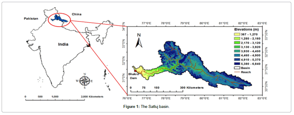
Figure 1: The Satluj basin.
Hydrometeorology in Satluj basin is defined by extremely complex biophysical environments produced by interactions among terrain, geology and meteorology. The basin experiences large variations in the climatic conditions ranging from the sub-tropical climate at the bottom of the Satluj valley to the alpine in the upper reaches, parts of which are perpetually under snow. Over 90% of the catchment lies above 1525 meters above mean sea level (masl) whereas the permanent snowline is at an elevation of 5400 m. The snow line descends to an elevation of about 2000 m by the end of winter with snow covering about 65% of the basin. It crosses 5000 m altitude by the end of the summer season with about 20% of the total drainage area remaining under perpetual snow and glaciers [33]. There is a large spatial variation in precipitation amount with many parts of the basin receiving heavy precipitation, whereas the Tibetan Plateau has a cold desert type climate with very little precipitation.
Data and Methodology
A well accepted method of assessing climatic impacts is through the analysis of hydrometeorological data. Analysis of temperature trends can provide critical evidence for evaluating impacts of anthropogenic climate change. In this paper, the focus is on the analysis of time series of surface air temperature, and various temperature indices for several stations in the Satluj River Basin. The dataset has been obtained from the India Meteorological Department (IMD) and Bhakra Beas Management Board (BBMB). Daily Minimum Temperature (TMN) and Maximum Temperature (TMX) data were available from 8 climate stations in the basin. The details of the meteorological stations are provided in Table 1 which shows station elevation and periods of record.
| S.No. | Station | Latitude | Longitude | Masl (m) | Data Availability | ||
|---|---|---|---|---|---|---|---|
| Degree | Minute | Degree | Minute | ||||
| 1 | Bhakra | 31 | 24 | 76 | 26 | 518 | 1974- 2010 |
| 2 | Kalpa | 31 | 32 | 78 | 15 | 2439 | 1984- 2010 |
| 3 | Kasol | 31 | 21 | 76 | 47 | 661 | 1964- 2008 |
| 4 | Kaza | 31 | 30 | 79 | 10 | 3639 | 1984- 2010 |
| 5 | Namgia | 31 | 48 | 78 | 39 | 2910 | 1985- 2010 |
| 6 | Raksham | 31 | 17 | 78 | 32 | 3130 | 1985- 2010 |
| 7 | Rampur | 31 | 26 | 77 | 38 | 1066 | 1972- 2010 |
| 8 | Suni | 31 | 15 | 77 | 7 | 625 | 1970- 2008 |
Table 1: Details of meteorological stations.
The analysis of trends has been carried out for a total number of 17 variables grouped in three sets (Table 2). Set A comprises variables based on annual values, whereas set B comprises variables based on seasonal values. Set C comprises variables describing the percentage of days when TMX and TMN are less than a predefined percentile (e.g, 10th and 90th percentile). The available daily surface air temperature data were used to derive the mean monthly data. The mean seasonal and annual series of all the variables for each station were then derived using the mean monthly data. The annual values of TMX in set A have been computed through averaging the mean monthly values of maximum temperature. The annual values of TMN have been computed by averaging the minimum temperature values over each year of the available data. The daily DTR has been computed by taking the difference between the daily TMX and TMN values. Using the daily DTR values, the annual values of DTR have been computed. The annual series of variables in set B (LTMX and LTMN) have been computed by extracting the largest and the smallest values of daily maximum and daily minimum temperature respectively for each year of the analysis period.
| Description | |
|---|---|
| Set A | |
| TMX | Annual average maximum temperature |
| TMN | Annual average minimum temperature |
| DTR | Annual average diurnal temperature range |
| WITMX | Maximum temperature averaged over winter |
| SPTMX | Maximum temperature averaged over spring |
| SUTMX | Maximum temperature averaged over summer |
| AUTMX | Maximum temperature averaged over autumn |
| WITMN | Minimum temperature averaged over winter |
| SPTMN | Minimum temperature averaged over spring |
| SUTMN | Minimum temperature averaged over summer |
| AUTMN | Minimum temperature averaged over autumn |
| Set B | |
| LTMX | Annual largest maximum temperature |
| LTMN | Annual largest minimum temperature |
| Set C | |
| TMX10 | percentage of days when TMX <10th percentile |
| TMX90 | percentage of days when TMX >90th percentile |
| TMX10 | percentage of days when TMN <10th percentile |
| TMX90 | percentage of days when TMN >90th percentile |
Table 2: List of variables.
In most land regions the frequency of warm days and warm nights will likely increase in the next decades, while that on cold days and cold nights will decrease [34]. To investigate the trends in the frequency of warm days, warm nights, cold days, and cold nights in the Satluj River basin, four temperature indices have been computed using the daily temperature data for each of the eight stations. A description of the temperature indices is provided in Table 2. TMN10 represents the percentage of days in a year when the TMN was less than the 10th percentile and is, therefore, an indicator of cold nights. TMX10 represents the percentage of days when TMX was less than the 10th percentile, and is, therefore, an indicator of cold days. Likewise, the variables TMN90 and TMX90 correspond to the 90th percentile and were similarly defined, and are indicators of warm nights and warm days respectively. To compute the annual series of variables in set C, the following procedure was adopted. For each year of the analysis period, the 10th and 90th percentiles of TMN were computed using 365 daily TMN values. Each of these 365 daily values was then compared with the 10th percentile value to determine the percentage of days when the daily TMN was less than the 10th percentile. Using this procedure, an annual time series of TMN10 was obtained. A similar procedure was adopted for TMN90. The procedure was repeated for TMX to obtain annual series of TMX10 and TMX90.
The trends in each of the variables described in Table 2 were investigated using Mann-Kendall nonparametric test [35,36]. Parametric tests are more powerful than the non-parametric ones, but the application of parametric tests requires that the data must be normally distributed. When the data are not normally distributed, nonparametric tests are considered more robust compared to their parametric counterparts. A major advantage of the Mann-Kendall test is that it allows missing data and can tolerate outliers. Several researchers have applied Mann-Kendall test to identify trends in the hydro-meteorological variables due to climate change [15,37]. The Mann Kendall test is a ranked based approach that consists of comparing each value of the time series with the remaining in a sequential order. The statistic S is the sum of all the counting as given in Equation (1).
 (1)
(1)
Where
 (2)
(2)
and xj and xk are the sequential data values, n is the length of the data set. A positive value of S indicates an upward and a negative value indicates a downward trend. For samples greater than 10, the test is conducted using normal distribution with the mean and variance as follows.
E[S] = 0(3)
 (4)
(4)
where, tp is the number of data points in the pth tied group and q is the number of tied groups in the data set. The standardized test statistic (Zmk) is calculated by:
(Zmk) is calculated by:
 (5)
(5)
where the value of Zmk is the Mann- Kendall test statistics that follows standard normal distribution with mean of zero and variance of one.
Trend evaluation using Mann-Kendall test relies on two important statistical metrics - the trend significance level or the p-value, and the trend slope ß. The p-value is an indicator of the trend significance – the lower the p-value the stronger is the trend. The metric ß provides the rate of change in the variable allowing determination of the total change during the analysis period. Using Sen’s slope method [38], the value of ß can be estimated. The method involves computing slopes for all the pairs of ordinal time points and then using the median of these slopes as an estimate of the overall slope. The Sen’s slope method is insensitive to outliers and can be effectively used to quantify a trend in the data. The presence of a positive serial correlation in a data set can increase the expected number of false positive outcomes for the Mann–Kendall test. A version of the Mann-Kendall test that incorporates the correction for serial correlation [39] has been used in this study.
Trend Results
The analysis of trends for the three sets of variables described in Table 2 has been carried out using Mann-Kendall nonparametric test. The statistical significance of trends is indicated by the p-value, and the magnitude and the direction of the trend has been computed using the Sen’s slope method. A value of 0.05 was chosen as a significance level for a two-sided test. Based upon this significance level, Zmk values greater than 1.96 or smaller than 1.96, respectively, indicate a significant positive or negative trend. A p-value of less than 0.05 indicates that the trend is statistically significant at 5% significance level. The bold values in the following tables indicate trends that are statistically significant at 5% significance level.
Trends in average temperature
A summary of trends in mean annual TMX, TMN, LTMX, LTMN, and DTR are presented in Table 3, where the bold values indicate statistically significant trends. The slope of the trend has the units of °C/year. The spatial distribution of trends in TMX and TMN is shown in Figure 2. Results presented in Table 3 clearly indicate that the positive trends outnumber the negative trends for all the variables. Of eight stations, six showed increasing trends in TMX with two exhibiting statistically significant trends. None of the stations showed statistically significant decreasing trends in TMX.
| Station | TMX | TMN | LTMX | LTMN | DTR | |||||
|---|---|---|---|---|---|---|---|---|---|---|
| Slope | p | Slope | p | Slope | p | Slope | p | Slope | p | |
| Bhakra | 0.021 | 0.289 | -0.022 | 0.024 | 0.036 | 0.089 | -0.091 | 0.001 | 0.042 | 0.102 |
| Kalpa | 0.04 | 0.073 | 0.032 | 0.07 | 0 | 0.866 | 0 | 0.521 | 0.015 | 0.307 |
| Kasol | -0.008 | 0.632 | -0.018 | 0.002 | 0 | 0.512 | -0.012 | 0.163 | 0.011 | 0.244 |
| Kaza | 0.091 | 0.067 | 0.096 | 0.027 | 0.042 | 0.187 | 0.056 | 0.661 | 0.017 | 0.739 |
| Namgia | 0.068 | 0.008 | 0.04 | 0.123 | 0 | 0.461 | 0 | 0.422 | 0.027 | 0.053 |
| Raksham | 0.059 | 0.026 | 0.077 | 0.001 | 0 | 0.964 | 0 | 0.799 | -0.01 | 0.523 |
| Rampur | 0.013 | 0.446 | 0.011 | 0.105 | 0.061 | 0.019 | 0 | 0.951 | 0.008 | 0.62 |
| Suni | -0.003 | 0.828 | -0.041 | 0.003 | 0.085 | 0.009 | 0 | 0.412 | 0.034 | 0.124 |
| No. + | 6 | 5 | 8 | 6 | 7 | |||||
| No. - | 2 | 3 | 0 | 2 | 1 | |||||
| No.Sig+ | 2 | 2 | 2 | 0 | 0 | |||||
| No.Sig - | 0 | 3 | 0 | 1 | 0 | |||||
2. Slope is in C/year
Table 3: Trends in Average Annual Temperature.
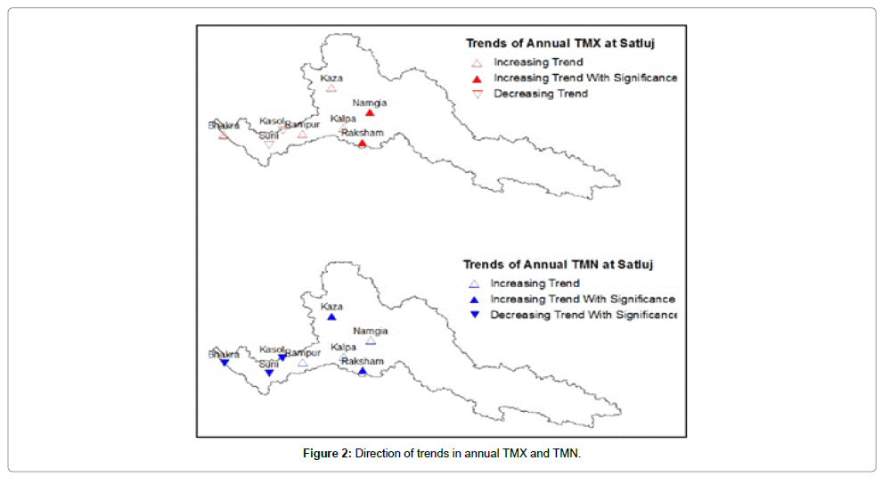
Figure 2: Direction of trends in annual TMX and TMN.
Mean annual TMN has shown a greater number of increasing trends than decreasing trends. Increasing trends were observed at five stations with two stations showing statistically significant trends. Bhakra showed an increasing trend in TMX (p=0.024) but it is not statistically significant (p=0.289). A statistically significant decreasing trend in TMN was, however, observed at Bhakra. In addition to Bhakra, Kasol (p=0.002) and Suni (p=0.003) exhibited strongly decreasing trends in TMN.
The trends in the time series of LTMX and LTMN were also investigated. For LTMX, all eight stations exhibited an increasing trend out of which two (Rampur and Suni) were statistically significant. The variable LTMN exhibited an increasing trend at six stations, but none of these were statistically significant. The decreasing trends in LTMN were observed at two stations, of which one was statistically significant (Bhakra, p=0. 001). The variable DTR showed an increasing trend at seven of the eight stations; none of the stations exhibited a statistically significant trend. The widening of DTR was expected due to an increasing trend in TMX and a decreasing trend in TMN observed at some stations.
Seasonal trends in TMX
Seasonal analysis of temperature data was carried out for the four seasons: winter (December-February), spring (March-May), summer (June-August), and autumn (September-November). The results of trend analysis of seasonal TMX are presented in Table 4, and spatial distribution of trends is shown in Figure 3. The trends in TMX for the winter season are predominantly increasing by six out of eight stations showing increasing trends with those at Kalpa and Namgia, being statistically significant. For the spring season, significantly increasing trends in TMX were found at four stations (Table 4 and Figure 3). None of the stations exhibited a statistically significant decreasing trend. For the summer season, increasing trend was found at six stations, and decreasing trend at two stations. None of the stations exhibited a statistically significant trend in the summer season. The autumn season, however, exhibited a greater number of decreasing trends than increasing trends, but an equal number of statistically significant decreasing and increasing trend (one each).
| Station | Winter | Spring | Summer | Autumn | ||||
|---|---|---|---|---|---|---|---|---|
| Slope | P | Slope | P | Slope | p | Slope | p | |
| Bhakra | 0.012 | 0.666 | 0.066 | 0.028 | 0.03 | 0.327 | -0.01 | 0.685 |
| Kalpa | 0.113 | 0.012 | 0.101 | 0.035 | -0.032 | 0.066 | 0.011 | 0.707 |
| Kasol | -0.024 | 0.153 | 0.03 | 0.18 | 0.006 | 0.487 | -0.03 | 0.05 |
| Kaza | 0.026 | 0.835 | 0.22 | 0.169 | 0.014 | 0.754 | 0.048 | 0.617 |
| Namgia | 0.127 | 0.045 | 0.184 | 0.006 | 0.018 | 0.35 | -0.002 | 1 |
| Raksham | 0.061 | 0.152 | 0.139 | 0.009 | -0.007 | 0.643 | 0.057 | 0.05 |
| Rampur | 0.028 | 0.143 | 0.051 | 0.066 | 0.019 | 0.384 | -0.03 | 0.217 |
| Suni | -0.023 | 0.276 | -0.006 | 0.681 | 0.051 | 0.093 | -0.029 | 0.204 |
| No. + | 6 | 7 | 6 | 3 | ||||
| No. - | 2 | 1 | 2 | 5 | ||||
| No.Sig+ | 2 | 4 | 0 | 1 | ||||
| No.Sig - | 0 | 0 | 0 | 1 | ||||
2. Slope is in C/year
Table 4: Trends in Seasonal Maximum Temperature.
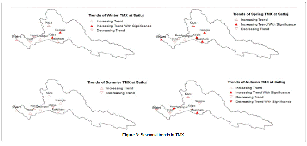
Figure 3: Seasonal trends in TMX.
Seasonal trends in TMN
| Station | Winter | Spring | Summer | Autumn | ||||
|---|---|---|---|---|---|---|---|---|
| Slope | p | Slope | P | Slope | p | Slope | p | |
| Bhakra | -0.033 | 0.002 | 0.012 | 0.685 | -0.024 | 0.015 | -0.024 | 0.024 |
| Kalpa | 0.062 | 0.055 | 0.062 | 0.017 | -0.012 | 0.532 | 0.003 | 0.77 |
| Kasol | -0.031 | 0.001 | -0.008 | 0.653 | -0.012 | 0.018 | -0.013 | 0.132 |
| Kaza | 0.035 | 0.359 | 0.185 | 0.175 | 0.01 | 0.934 | 0.088 | 0.416 |
| Namgia | 0.047 | 0.272 | 0.062 | 0.076 | 0.046 | 0.019 | 0.027 | 0.224 |
| Raksham | 0.153 | 0.001 | 0.101 | 0.004 | 0.023 | 0.179 | 0.032 | 0.094 |
| Rampur | 0.008 | 0.377 | 0.022 | 0.157 | 0.023 | 0.075 | 0.005 | 0.594 |
| Suni | -0.062 | 0.005 | -0.06 | 0.005 | -0.022 | 0.045 | -0.027 | 0.147 |
| No. + | 5 | 6 | 4 | 5 | ||||
| No. - | 3 | 2 | 4 | 3 | ||||
| No.Sig+ | 1 | 2 | 1 | 1 | ||||
| No.Sig - | 3 | 1 | 3 | 0 | ||||
2. Slope is in C/year
Table 5: Trends in Seasonal Minimum Temperature.
Seasonal trends in TMN are shown in Table 5 and the spatial distribution in Figure 4. For the winter season, three statistically significant decreasing trends for TMN were found, although no significant decreasing trends were found for TMX. For the spring season, three stations exhibited statistically significant increasing trend, whereas one exhibited statistically significant decreasing trend. There were an equal number of stations exhibiting increasing and decreasing trends for the summer season. However, the number of stations exhibiting statistically significant decreasing trend is more than the number of stations with an increasing trend. For the autumn season, although there were five increasing trends, but only one was statistically significant with a p-value of 0.094. Out of three decreasing trends, only one (Bhakra) was statistically significant.
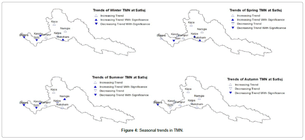
Figure 4: Seasonal trends in TMN.
Trends in temperature indices
Table 6 shows the results of trends in four temperature indices considered. For each of the four temperature indices, increasing trends outnumbers the decreasing trends. The variable TMX10 showed an increasing trend at five stations (three significant) and decreasing trends (one significant) at three stations. The trends in TMX90 are similar to those for TMX10 with six stations exhibiting increasing trend, but none of these were statistically significant thus indicating weak increasing trends in maximum daytime temperature. Two stations exhibited decreasing trends of which Suni had a statistically significant trend. Suni is the only station that showed a statistically significant decreasing trend in both TMX10 and TMX90. For TMN10, the number of stations with increasing trends is equal to the number of stations with decreasing trends. The only station that showed a statistically significant trend in TMN10 was Bhakra, but none of the stations exhibited statistically significant decreasing trend. For TMN90, equal numbers of increasing and decreasing trends were obtained but none of these trends were statistically significant.
| Station | TMX10 | TMX90 | TMN10 | TMN90 | ||||
|---|---|---|---|---|---|---|---|---|
| Slope | P | Slope | P | Slope | P | Slope | P | |
| Bhakra | 0.017 | 0.237 | 0.001 | 0.843 | 0.049 | 0.015 | 0.001 | 0.591 |
| Kalpa | 0.001 | 0.584 | -0.012 | 0.543 | -0.017 | 0.439 | 0.004 | 0.615 |
| Kasol | 0.011 | 0.247 | 0.007 | 0.48 | 0.001 | 0.637 | -0.001 | 0.61 |
| Kaza | 0.001 | 0.883 | 0.001 | 0.601 | 0.001 | 0.691 | -0.002 | 0.615 |
| Namgia | -0.048 | 0.744 | 0.001 | 0.851 | -0.097 | 0.575 | 0.001 | 0.705 |
| Raksham | 0.035 | 0.033 | 0.001 | 0.894 | 0.001 | 0.627 | 0.007 | 0.724 |
| Rampur | -0.017 | 0.156 | 0.001 | 0.762 | -0.015 | 0.505 | -0.018 | 0.388 |
| Suni | -0.024 | 0.025 | -0.036 | 0.006 | -0.046 | 0.067 | -0.049 | 0.099 |
| No. + | 5 | 6 | 4 | 4 | ||||
| No. - | 3 | 2 | 4 | 4 | ||||
| No. Sig+ | 1 | 0 | 1 | 0 | ||||
| No. Sig- | 1 | 1 | 0 | 0 | ||||
2. Slope is in C/year
Table 6: Trends in Temperature Indices.
Discussion and Conclusions
Long term trends of seasonal and annual temperatures, both maximum and minimum, have been investigated using Mann-Kendall nonparametric test. Additionally, trends in DTR, LTMX, LTMN, and four temperature indices have been investigated for eight stations in the Satluj River Basin. The intention behind the analysis conducted in this research was to assist, through interpretation of trends, in the development of adaptation strategies to counteract the adverse impacts of climate change in the basin that is considered to be highly vulnerable to the impacts of global warming. The version of the Mann-Kendall test applied herein alleviates some of the problems in trend analysis of historical data with the intent of establishing a research agenda that can further address issues of global warming.
A clear warming pattern was observed in the basin with the majority of the stations (six of eight) exhibiting increasing trends in annual TMX. None of the stations exhibited a statistically significant decreasing trend in annual TMX. The trends in annual TMN were, however, mixed with a bias towards increasing trends. However, three stations showed statistically significant decreasing trends in TMN. The observed cooling trend at these stations in the basin corresponds with results for minimum temperature reported by Fowler and Archer [40] for the upper Indus Basin. The predominantly increasing trend in diurnal temperature range owing to the asymmetrical trends in TMX and TMN is also shared with upper Indus stations [41] and has also been reported in parts of India [42]. This contradicts general global patterns whereby faster increases in TMX than TMN yield decreasing DTR [27,43].
Some higher elevation stations (for example, Raksham, Kaza, and Namgia) showed clear warming trends both in TMX and TMN. Similar findings have been reported in some studies on the Himalayas in Xizang province of China, which found higher warming rates at higher altitudes [44-49]. Increased warming in the higher elevation stations is likely to result in increased melting of glaciers and snowfields. This could have a serious impact on water availability in the basin as higher volume of water would be available downstream during the first half of this century, but acute shortages may occur in water availability during the second half of the current century with diminished glacier and snowfield extent. The underlying assumption for this plausible scenario is that the current temperature trends will continue in the future.
Trend analysis of seasonal temperature data revealed that the warming was more pronounced in winter and spring seasons than in summer and autumn seasons. This melt during the spring months may be especially enhanced, but may be less serious during the summer months. Trends in all four temperature indices considered in this study were predominantly increasing. For TMX90, there were eight increasing trends whereas TMN90 exhibited seven increasing trends. At four stations, TMN90 exhibited increasing trends with very low p-values. The lower the p-values the stronger is the trend, and; therefore, a clear warming trend in nighttime temperature represented by TMN90 was found from the analysis.
Analysis of results clearly revealed a greater number of increasing trends in most of the variables investigated than could be expected to occur by chance. The general pattern in the trends clearly indicated increased warming in the basin, which could have implications for water availability in the basin as the contribution of snow and glacier melt to annual runoff at Bhakra reservoir is about 60%. If the current trends in temperature continue in the future, the magnitude and timings of water availability at Bhakra reservoir could be significantly impacted thereby putting drinking water supplies of millions of people at risk. It may be concluded that the analysis of historic temperature data in India indicates predominantly increasing trends, but not uniformly so by season, by region or between the maximum and minimum temperature. However, the analysis conducted in the present work depends upon the quality of data.
A well-known limitation of trend analysis of historical data is that the analysis is, by its nature, retrospective. Of greater concern from an engineering design perspective is what conditions can be expected to occur in the future, particularly within the design life of a given piece of infrastructure. A purely retrospective analysis of the available data may not be a good indicator of future conditions. To obtain a more comprehensive view of the present and plausible future conditions in the basin requires combining trend analysis of historical data with analysis of climate data obtained from modelling climate change projections using downscaled results from Global Climate Models (GCMs) in conjunction with an appropriate hydrological model. A second limitation of the present research is that the hydro-meteorological data used in the trend analysis are available up to 2010. More recent data are not available. The trend analysis carried out in this research would have been more reliable had the recent data been available from a greater number of stations as climate change impacts are believed to be more pronounced during the recent period.
Acknowledgements
The authors acknowledge the support by Ministry of higher education and scientific research of Iraq, the University of Mosul, Mosul, Iraq and the Indian Council for Cultural Relations (ICCR), India.
References
- IPCC (2007a) Impacts, Adaptation and Vulnerability. Asia Climate Change 2007. Parry ML, Canziani OF, Palutikof JP, van der Linden PJ, Hanson CE (edn). Cambridge University Press, Cambridge, UK 469-506.
- IPCC (2007b) Intergovernmental Panel on Climate Change. Summary for policymakers. Solomon S, Qin D, Manning M, Chen Z, Marquis M, et (edn). Climate change 2007: the physical science basis. Cambridge University Press, Cambridge 13-14.
- Khattak MS, Babel MS, Sharif M (2011) Hydro-meteorological trends in the upper Indus River basin in Pakistan. Clim Res 46: 103-119.
- Ramanathan V, Chung C, Kim D, Bettge T, Buja L, et al. (2005) Atmospheric brown clouds: Impacts on South Asian climate and hydrological cycle. Proc Nat AcadSci USA 102: 5326-5333.
- Jones PD, Moberg A (2003) Hemispheric and large-scale surface air temperature variations: An extensive revision and an update to 2001. J Climate 16: 206-223.
- Ohmura A (2012) Enhanced temperature variability in high-altitude climate change. TheorApplClimatol 110: 499-508.
- Yang F, A Kumar ME, Schlesinger, Wang W (2003) Intensity of hydrological cycles in warmer climates. J Climate 16: 2419-2423.
- Simonovic SP, Li L (2003) Methodology for assessment of climate change impacts on large-scale flood protection system. J Water Resour Plan Manage 129: 361-372.
- Jiang T, Chen YD, Xu CY, Chen X, Singh VP (2007) Comparison of hydrological impacts of climate change simulated by six hydrological models in the Dongjiang basin, South China. J Hydrol 336: 316-333.
- Hingane LS, Rup Kumar K, Ramanamurthy BV (1985) Long term needs of surface air temperature in India. Int J Climatol 5: 521-528.
- Rao PG (1993) Climatic changes and trends over a major river basin in India. Clim Res 2: 215-223.
- Sinha Ray KC, Mukhopadhya RK, Chowdhary SK (1997) Trend in maximum and minimum temperature and sea level pressure over India. INTROMET 1997 IIT Delhi, HauzKhas, New Delhi.
- Pant GB, Kumar KR (1997) Climates of South Asia. John Wiley and Sons Ltd., Chichester, UK.
- Arora M, Goel NK, Singh R (2005) Evaluation of temperature trends over India. HydrolSci J 50: 81-93.
- Singh P, Kumar V, Thomas T, Arora M (2008) Basin-wide assessment of temperature trends in northwest and central India. HydrolSci J 53: 421-433.
- Cheema MA, Farooq M, Ahmad R, Munir H (2006) Climatic trends in Faisalabad (Pakistan) over the last 60 years (1945-2004). J AgriSocSci 2: 42-45.
- Barnett TP, Adam JC, Lettenmaier DP (2005) Potential Impacts of a Warming Climate on Water Availability in Snow-dominated Regions. Nature 438: 303-309.
- Xu KM, Zhang M, Eitzen ZA, Ghan SJ, Klein SA, et al. (2005) Modeling springtime shallow frontal clouds with cloud-resolving and single-column models. J Geophys Res 110.
- Schild A (2008) ICIMOD’s position on climate change and mountain systems. Mountain Res Develop 28: 328-331.
- Government of India (GOI) (2012) Status of hydroelectric potential development.
- Cruz RV, Harasawa H, Lal M, Wu S, Anokhin Y, et al. (2007) Asia. Climate Change 2007: Impacts, Adaptation and Vulnerability. Parry ML, Canziani OF, Palutikof JP, Van Der Linden PJ, Hanson CE (edn). Contribution of Working Group II to the Fourth Assessment Report of the Intergovernmental Panel on Climate Change. Cambridge University Press, Cambridge, UK 469-506.
- Rathore BP, Kulkarni AV, Sherasia NK (2009) Understanding future changes in snow and glacier melt runoff due to global warming in Wangar Gad Basin, India. CurrSci 97: 1077-1081.
- Shrestha AB, Wake CP, Mayewski PA, Dibb JE (1999) Maximum temperature trends in the Himalaya and its vicinity: an analysis based on temperature records from Nepal for the period 1971-94. J Climate 12: 2775-2786.
- Cook ER, Krusic PJ, Jones PD (2003) Dendroclimatic signals in long tree-ring chronologies from the Himalayas of Nepal. Int J Climatol 23: 707-732.
- Shrestha AB, Wake CP, Dibb JE, Mayewski PA (2000) Precipitation fluctuations in the Nepal Himalaya and its vicinity and relationship with some large scale climatological parameters. Int J Climatol 20: 317-327.
- Fowler HJ, Archer DR (2005) Hydro-climatological variability in the upper Indus Basin and Implications for water resources. In: Wagener T, et al. (edn), Regional Hydrological Impacts of Climatic Change – Impact Assessment and Decision Making. IAHS Publ 295: 131-138.
- Easterling DR, Horton B, Jones PD, Peterson TC, Karl TR, et al. (1997) Maximum and minimum temperature trends for the globe. Sci 277: 364-367.
- Jones PD, New M, Parker DE, Martin S, Rigor IG (1999) Surface air temperature and its variations over the last 150 years. Rev Geophys 37: 173-199.
- Dash SK, Jenamani RK, Kalsi SR, Panda SK (2007) Some Evidence of Climate Change in Twentieth-century India. Climatic Change 85: 299-321.
- Dimri AP, Dash SK (2011) Winter time climatic trends in the Western Himalayas. Climatic Change 111: 775-800.
- Immerzeel W (2008) Historical trends and future predictions of climate variability in the Brahmaputra Basin. Int J Climatol 28: 243-254.
- Viviroli D, Archer DR, Buytaert W, Fowler HJ, Greenwood GB, et al. (2011) Climate change and mountain water resources: overview and recommendations for research, management and policy. Hydrol Earth Syst Sci 15: 471-504.
- Singh P, Jain SK (2002) Snow and glacier melt in the Satluj River at Bhakra Dam in the Western Himalayan region. HydrolSci J 47: 93-106.
- Kirtman B, Power SB, Adedoyin JA, Boer GJ, Bojariu R, et al. (2013) Near-term Climate Change: Projections and Predictability. In: Climate Change 2013: The Physical Science Basis. Contribution of Working Group I to the Fifth Assessment Report of the Intergovernmental Panel on Climate Change. Stocker TF, Qin D, Plattner GK, Tignor M, Allen SK, et al. (edn). Cambridge University Press, Cambridge, United Kingdom and New York, NY, USA.
- Mann HB (1945) Non-parametric tests against trend. Econometrica 13: 245-259.
- BurnDH, Sharif M, Zhang K (2010) Detection of trends in hydrological extremes for Canadian watersheds. HydrolProc 24: 1781-1790.
- Sen PK (1968) Estimates of the regression coefficient based on Kendall’s tau. J Am Stat Assoc 63: 1379-1389.
- Yue S, Pilon PJ, Phinney B, Cavadias G (2002) The influence of autocorrelation on the ability to detect trend in hydrological series. HydrolProc 16: 1807-1829.
- Fowler HJ, Archer DR (2006) Conflicting Signals of Climate Change in the Upper Indus Basin. J Climate 19: 4276-4292.
- Forsythe N, Kilsby CG, Fowler HJ, Archer DR (2012) Assessment of runoff sensitivity in the Upper Indus Basin to inter annual climate variability and potential change using MODIS satellite data products. Mountain Res Develop 32: 16-29.
- Kumar KR, Kumar KK, Pant GB (1994) Diurnal asymmetry of surface temperature trends over India. Geophys Res Lett 21: 677-680.
- Karl TR, Knight RW, Gallo KP, Peterson TC, Jones PD, et al. (1993) A new perspective on recent global warming- Asymmetric trends of daily maximum and minimum temperature. Bull Amer Meteor Soc 74: 1007-1023.
- Liu X, Cheng Z, Yan L, Yin ZY (2009) Elevation dependency of recent and future minimum surface air temperature trends in the Tibetan Plateau and Its surroundings. Global Planet Change 68: 164-174.
- Liu X, Chen B (2000) Climatic Warming in the Tibetan Plateau during recent decades. Int J Climatol 20: 1729-1742.
- Qin J, Yang K, Liang S, Guo X (2009) The altitudinal dependence of recent rapid warming over the Tibetan Plateau. Climatic Change 97: 321-327.
- Thompson LG, Mosley-Thompson E, Davis ME, Lin PN, Henderson K, et al. (2003) Tropical glacier and ice core evidence of climate change on annual to millennial time scales. Climatic Change 59: 137-155.
- Yang X, Zhang T, Qin D, Kang S, Qin X (2011) Characteristics and changes in air temperature and glacier’s response on the north slope of MT. Qomolangma (Mt. Everest). Arctic, Antarctic, and Alpine Research 43: 147-160.
- Vorosmarty CJ, McIntyre PB, Gessner MO, Dudgeon D, Prusevich A, et al. (2010) Global threats to human water security and river biodiversity. Nature 467: 555- 561.
Citation: Hamid AT, Sharif M, Archer D (2014) Analysis of Temperature Trends in Satluj River Basin, India. J Earth Sci Clim Change 5: 222. DOI: 10.4172/2157-7617.1000222
Copyright: ©2014 Hamid AT, et al. This is an open-access article distributed under the terms of the Creative Commons Attribution License, which permits unrestricted use, distribution, and reproduction in any medium, provided the original author and source are credited.
Select your language of interest to view the total content in your interested language
Share This Article
Recommended Journals
Open Access Journals
Article Tools
Article Usage
- Total views: 18242
- [From(publication date): 10-2014 - Aug 30, 2025]
- Breakdown by view type
- HTML page views: 13387
- PDF downloads: 4855