Climate Change Impact on Drought Intensity and Duration in West of Iran
Received: 14-Aug-2015 / Accepted Date: 21-Sep-2015 / Published Date: 30-Sep-2015 DOI: 10.4172/2157-7617.1000319
Abstract
In this paper, one of the probabilistic characterizations of drought events (i. e. intensity values) was simulated by a global climate model (GCMs) under enhanced greenhouse gases conditions for near future (2011-2030). Output of the Hadley Centre Global Climate Model (HadCM3) was used to provide a future climate scenario for precipitation in selected western stations of Iran, including Ilam, Hamedan, Kermanshah, KhoramAbad, Sanandaj, Zanjan. Because of the coarse resolution of GCM output model, a statistical downscaling method, LARS_WG, was applied in order to obtain site specific daily weather Series. The downscaling model was evaluated against available observational reference data (1961-1990). The performance of LARS-WG during the validation period was suitable to reproduce daily precipitation series, therefore this model was used to provide future scenario of daily precipitation for 2011-2030 period. The simulation was forced by the A1B, B2 and A2 emission scenario for HadCM3. SPI was calculated using the downscaled precipitation time series for baseline and near future period. The model also captures the properties of drought for baseline acceptably. The results show that the future amounts of precipitation do not differ significantly in comparison with baseline. The most percentage change is obtained by 28% in the Kermanshah station Under B1 emission scenario during near future, but the increase is not significant. SPI was calculated for long-time drought (12 months) and then 2, 5, 10, 20, 25, 50, 100 return periods were estimated for all stations. Based on the results, the severity of drought will increase with longer return period i. e. 100 years in Kermanshah, Zanjan and Khoram Abad Stations. This information was achieved by this research can be considered indicative in long-term planning focusing on sustainability.
Keywords: Drought; Standard precipitation index; Return period
10127Introduction
Successful management of water in the event of drought requires understanding its causes and processes. Several definitions have been provided for drought, which are mainly dependent on the views of water consumers and managers. Here, drought is defined as an abnormal and temporary imbalance in water resources, and includes precipitation constantly less than average and with unknown frequency, duration, and intensity, making difficult or impossible to predict its occurrence; this reduces available water resources and the capacity of ecosystems maintenance. It is important to understand low capability of drought prediction, turning it into a hazard and a disaster: a hazard, since drought is an unpredictable natural event with imminent return, and a disaster, because the failure of precipitation regime results in water scarcity and affects agricultural and natural ecosystems and other human activities. Hazardous and disastrous nature of drought necessitates development of a variety of tools for its prediction, including various probabilities; this can support early warning systems for timely preparedness and mitigation of damages. Drought begins slowly and is felt at the time of event. It lasts for long periods, usually affect large areas, and its effect is pervasive. It is very difficult to predict the onset and end of drought. The exact time interval between the publication of prediction and the actual start of the predicted drought is often more important than the prediction accuracy. This interval provides an opportunity for decision- and policy-makers to take timely measures to mitigate the effects of drought [1]. Recent reports of Intergovernmental Panel on Climate Change (IPCC) indicated the increased frequency and severity of extreme climatic events during climate change, so that increase in greenhouse gases and global warming will manifest as an increase in the intensity and frequency of extreme climatic events such as extreme precipitation, drought, and flood (WMO). In such circumstances, economic development and sustainable living conditions in the coming years is related to the ability to manage risks relevant to extreme events [2]. In this context, any attempt to predict extreme events, including droughts and floods in any region seems essential. In the past century, a number of indices have been provided for quantifying, monitoring, and analyzing droughts, and attempts have also been made to improve and present new indices [3-5]. Regarding the analysis of drought and establishment of a monitoring system, most studies employ the Palmer Drought Severity Index (PDSI) [6] and the Standardized Precipitation Index (SPI). The former is based on the soil-water balance equation and the later on the probability of precipitation [7]. SPI has been widely used in the research on drought in Iran and throughout the world, since it can be calculated with a low number of data (only precipitation). SPI does not consider other variables affecting drought such as temperature, evapotranspiration, wind speed, soil, and water holding capacity, however several studies have shown that precipitation is the main variable in determining the onset, duration, intensity, and the end of drought [4]. Therefore, low diversity of data required and their simplicity are the reasons for the widespread use of this index for monitoring and analysis of drought. Regarding the issue of climate change and to predict changes in the intensity and frequency of extremes, it is necessary to produce climate scenarios. In addition, in order to study the effect of climate change on water resources in future periods and generation of scenarios for extreme precipitation amounts, climatic variables should be simulated under the impact of changes in greenhouse gases. Various methods have been introduced for simulation of climate variables in future periods under the impact of climate change; the most valuable of them uses General Circulation Models (GCMs) [8]. As the most reliable source for climatic data at present, GCMs are capable of reproducing the main atmospheric processes at a global and continental scale and predict climate under different scenarios. The new generation of these models has been provided as Atmospheric-Ocean General Circulation Model (AOGCM) which is able to precisely and completely simulate the climate system. Numerous GCMs have been designed in various research centers, such as HadCM3, ECHAM4, CSIRO, CGCM2, and ECHO-G. Since the amount of greenhouse gas emission in future periods is the most important input to these models, various emission scenarios have been proposed involving the mode of changes in these gases in the future [9]. Scenarios of future especial emission of greenhouse gases are utilized to assess the potential effects of increased greenhouse gases on the frequency and severity of droughts in the future. Many studies have been carried out so far to provide scenarios of future temperature, precipitation, and extreme events such as drought using climate model outputs. Jiang [10] used data from 550 stations in China during 1961-2000 to evaluate seven AOGCMs for simulation of extreme temperature and precipitation indices. The findings showed that the models were capable of simulating the process and distribution of extreme climate events. In this regard, Seilman [11] estimated the indices of precipitation and temperature using the ECHAM5 output model. The results indicated that heat waves and the maximum number of consecutive dry days increase and the total number of frost days reduce in the future periods. Semenov [12] analyzed changes in the magnitude and temporal patterns of two extreme indices for wheat, including the probability of thermal stress during flowering and the severity of drought stress. In order to calculate this index, a wheat simulation model was used along with the scenarios based on the output of HadRM3 in 18 stations in England and Wales (downscaled by LARS-WG model). The results showed that despite higher temperature and lower summer precipitation forecasted for the period of 2050, the effect of drought stress on wheat yield was predicted to be less than the current period, because wheat ripens sooner to escape the summer drought stress. But the damage caused by heat stress during flowering increased significantly during this period. Golmohammadi and Massah [13] studied the average precipitation of 11 stations in Gharehsou basin during the baseline period of 1971-2000. They used precipitation from HadCM3 under the A2 scenario for the period of 2040-2069, and identified SPI for different time scales of 6, 12, and 24 months and drought conditions in Gharehsou basin for different return periods during this period. Comparison of the results showed that precipitation will be increased in the basin during this period, resulting in declined severity of the drought compared to the baseline. With an increase in the return period, the reduced intensity increases in the time scale of 6 and 12 months. While for the drought period of 24 months, the severity of drought in the basin will be higher than the baseline period with an increase in the return period [13].
Fattahi and Sedaghat Kerdar determined the persistence, intensity, and frequency of drought for time scales of 3, 6, 12, 24, and 48 months, using data from total monthly precipitation obtained from the synoptic stations in western basins of Iran during the period of 1960-2000, and utilizing time series of standardized precipitation index. The results showed that drought occurred when the index had negative sequences, and the drought intensified when the values of SPI were -1 or less. Aiming at establishing a relationship between the occurrence of drought in different areas using SPI, LashniZand and Telvari [14] prepared monthly drought maps for a period of thirty years, and predicted climatic drought of the next 48 months for each basin and the whole region. Razii [15] studied the intensity, persistence, and frequency of meteorological drought in Sistan and Baluchestan Province through combining RUN theory and Markov chain, and making the transition probability matrix and the static matrix, and predicted the persistence and duration of droughts over the next 10 years. Aiming at zoning drought, Nasri [16] studied two features of drought including the possibility of severe drought and its duration on 34 synoptic stations in central Iran. The results showed that drought in eastern and southwestern regions had higher intensity. Lou Alizadeh [17] evaluated the droughts of Ahwaz in terms of intensity, persistence, and frequency using the standardized precipitation index at the periods of 12 and 24 months. To this end, the monthly precipitation data of 45 years from synoptic station of Ahwaz were studied which showed that the duration and severity of droughts during 2001-2011 increased compared with the past 4 decades.
Materials And Methods
Drought is a stochastic-probabilistic and unpredictable phenomenon, but when occurred, it persists for a long time. Drought has been defined quantitatively in many ways, including the Run approach which investigates the stochastic characteristics of time series, and drought indices. Some indices have been introduced by meteorologists and hydrologists for monitoring and predicting drought. These indices rely on either the climatic-hydrologic variables or the occurrence of drought. The drought indices with one or more than one variable are mainly used for monitoring drought at different time scales. Palmer Drought Severity Index (PDSI) [6]. And Standard Precipitation Index (SPI) [7,18] are two examples of these indices which can be calculated with the data obtained from weather stations.
Standardized Precipitation Index (SPI)
To monitor and manage water resources, drought indices should be associated with specific time scale and should be comparable in temporal and spatial scale, making them usable for monitoring drought at various time intervals [19]. In this regard, introduced SPI for quantification of precipitation deficit at multiple time scales [7]. Drought is a multi-scale phenomenon [7]. Clearly showed that drought is a multi-scale phenomenon comprising soil moisture, groundwater, snow, and water withdrawal from rivers and reservoirs. Thus, time scale greatly affects the accumulated water scarcity and accordingly, drought can be characterized separately in terms of hydrology, environment, agriculture, and so on. For this reason, drought indices should be associated with a specific time scale to be useful for monitoring and management of water resources. This description justifies the extensive acceptance of SPI, as a temporally and spatially comparable index, which can be calculated for different time scales for drought monitoring, according to various available resources of water [19]. SPI only uses rainfall data and makes possible to calculate the amount of cumulative precipitation at multiple time scales using a shifting window. SPI is widely used due to easy, reliable, and relative comparison between different locations and climates. Evaluated the application of this index in describing the drought in Hungry [20]. They concluded that SPI is suitable for qualification of most types of drought [21,22]. Applied SPEI and SPI for monitoring drought at multiple time scales in eastern California and Nevada and concluded that both indices were significantly correlated with variations in river runoff. In other research aiming at evaluating the performance of different drought indices, predicting changes in runoff, soil moisture, forest growth, and crop yield were compared using three indices of PDSI, SPI, and SPEI. The results showed that the efficiency of SPEI and SPI for detection of drought based on hydrological, agricultural, and environmental variables was higher than PDSI in different time scales [23]. For each location, SPI is calculated using long-term records for the period in question. These data are fitted with a probability distribution and then converted to a normal distribution, so that the mean SPI for any region is zero during the studied period [24] (Table 1). Developed the Standardized Precipitation Index (SPI) for the purpose of defining and monitoring drought among others, the Colorado Climate Center, the Western Regional Climate Center, and the National Drought Mitigation Center use the SPI to monitor current states of drought in the United States [7]. The nature of the SPI allows an analyst to determine the rarity of a drought or an anomalously wet event at a particular time scale for any location in the world that has a precipitation record found the gamma distribution to fit climatological precipitation time series well. The gamma distribution is defined by its frequency or probability density function:
| Condition | Cumulative Probability | SPI |
|---|---|---|
| Extremely drought | 0.0014 | -3.0 |
| Very severe drought | 0.0062 | -2.5 |
| Severe drought | 0.0228 | -2.0 |
| Moderately drought | 0.0668 | -1.5 |
| Mildly drought | 0.1587 | -1.0 |
| Nearly normal | 0.3085 | -0.5 |
| Normal | 0.50 | 0 |
| Nearly normal | 0.6915 | 0.5 |
| Mildly wet | 0.8413 | 1.0 |
| Moderately wet | 0.9332 | 1.5 |
| Severe wet | 0.9772 | 2.0 |
| Very severe wet | 0.9938 | 2.5 |
| Extremely wet | 0.9986 | 3.0 |
Table 1: Classification of drought using SPI values and probabilities associated with each event [18] Formed and fitted to the time series distribution.
For x>01)
Where:
α> 0 α is a shape parameter
β >0 β is a scale parameter
x> 0 x is the precipitation amount
Computation of the SPI involves fitting a gamma probability density function to a given frequency distribution of precipitation totals for a station. The alpha and beta parameters of the gamma probability density function are estimated for each station, for each time scale of interest (3 months, 12 months, 48 months, etc.), and for each month of the year. The maximum likelihood solutions are used to optimally estimate α and β:

Where:
n = number of precipitation observations
 = Cumulative average rainfall for a month during the statistical period
The resulting parameters are then used to find the cumulative probability of an observed precipitation event for the given month and time scale for the station in question.
Letting  this equation becomes the incomplete gamma function:

Since the gamma function is undefined for x=0 and a precipitation distribution may contain zeros, the cumulative probability becomes:
Where eqn is the probability of a zero. The cumulative probability, H(x), is then transformed to the standard normal random variable Z with mean zero and variance of one, which is the value of the SPI. That converts cumulative probability to the standard normal random variable Z.
0<H(x) ≤0.5 
0.5<H(x)
where:
0<H(x) ≤0.5 
0.5<H(x)
The coefficient is equal to:


Thus SPI indicates the z score that the value of the normalized deviations above or below the mean of the show.
Hadley coupled atmosphere-ocean general circulation model (HadCM3)
This model was designed and developed at the Hadley Centre, UK. It was described by Gordon et al., [25] and HadCM3 consists of two atmospheric (HadAM3) and oceanic (HadOM3) components. IPCC has used HadCM3 data of general circulation model for preparation of the third report. Simulations are done based on a 360 days a year and 30 days a month calendar. High resolution of the oceanic component is the main advantage of this model. A good coordination between the atmospheric and oceanic components is another advantage of this model [26].
LARS-WG
Low spatial and temporal resolution of general circulation models of atmosphere and uncertainty in their daily outputs especially precipitation have made inappropriate the direct use of these outputs in analysis of extreme events and their application in different models [12]. Therefore, to use these data, the models outputs at the station level should be downscaled through various techniques. Downscaling methods include dynamic downscaling using regional climate models such as REGCM, statistical downscaling such as ASD and SDSM models, and stochastic weather generator models such as LARSWG [12]. The latter is the most widely used statistical model for downscaling the outputs of GCMs. The first version of LARS-WG was developed in Budapest, Hungary, in 1991 as a part of an agricultural project risk assessment. The main objective of this approach was to overcome the limitations of the Markov chain method in precipitation. The effectiveness of this model was evaluated by Semenov at 18 stations in the US, Europe, and Asia in 1998 [27].
The Semi-Empirical Distribution (SED) model is used to estimate the probability distribution of wet and dry series, daily precipitation, maximum and minimum temperature, and solar radiation. This distribution is determined as the cumulative probability distribution function. An amount of climate variables (vi) is calculated for each climate variable (v) corresponding to the probability of pi as follows:
 (1)
(1)
In this equation P() represents the probability based on the observational data {vobs}. Two values of p0 and pn are determined for each climate variable as p0=0 and pn=1 corresponding to v0=min{vobs} and vn=max{vobs}. To exactly approximate the extreme values of any climate variable, the value of pi is determined for very low values, close to zero, and very high values of variables. The remaining values of pi are evenly distributed according to probabilistic weight. Three values near 1 are used for precipitation (pn-1=0.999, pn-2=0.995, and pn-3=0.985). These values allow a better approximation of daily precipitation extreme events that occur with very small probability (such as rainfall during storms). The number of intervals used in SED version 5 is 23, providing an exact observed distribution compared with the previous version (with an interval of 10) [9]. The amount of rainfall for a wet day (with precipitation greater than zero mm) is calculated using a semiempirical distribution. Daily maximum and minimum temperature is estimated according to wetness or dryness of the desired day. Maximum and minimum daily temperatures are modeled considering the daily mean and standard deviation through statistical process.
Data
In this study, monthly and daily precipitation data were collected from 6 stations. Characteristics and locations of the stations are depicted in Table 2 and Figure 1, respectively. They were selected according to the availability of precipitation data, proper regional distribution, and concurrency of the stations data in a statistical period of more than ten years which ranged between 20 and 30 years (Figure 1).
| Station | Latitude | Longitude | Altitude (m) |
|---|---|---|---|
| Ilam | 33° 38’ | 46° 26’ | 1337 |
| Khorramabad | 33° 26’ | 48° 17’ | 1147.8 |
| Zanjan | 36° 41’ | 48° 29’ | 1663 |
| Sanandaj | 35° 20’ | 47° 00’ | 1373.4 |
| Kermanshah | 34° 21’ | 47° 09’ | 1318.6 |
| Hamedan | 34° 52’ | 48° 32’ | 1741.5 |
Table 2: Geographical coordinates of the studied stations.
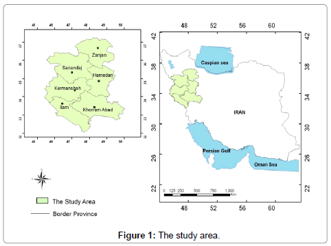
Figure 1: The study area.
Results
Calculation of SPI and drought return periods
To calculate SPI for the baseline period, the monthly precipitation data of the studied stations in the available period (1961-1990) were obtained from the National I.R. of Iran Meteorological Organization. The data were then used to prepare the input file for the SPI software after being ensured of their homogeneity. Then drought index was calculated for 1, 3, 6, and 12 timescales. Figures 2-8 present SPI at a 12-month timescale during baseline period of each station. According to the drought classification table as well as the study objectives, drought events (less than -1) were obtained at a 12-month scale. Hyfa was utilized to obtain the drought values in return periods of 2, 5, 10, 20, 50 and 100 years.
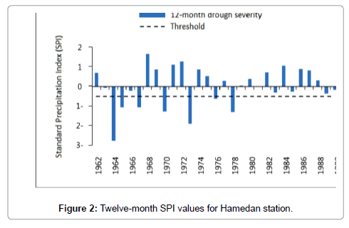
Figure 2: Twelve-month SPI values for Hamedan station.
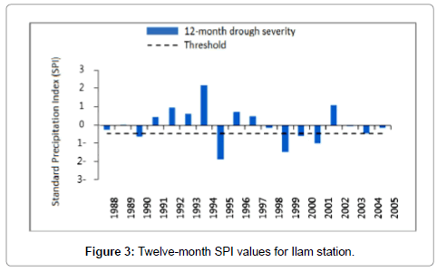
Figure 3: Twelve-month SPI values for Ilam station.
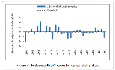
Figure 4: Twelve-month SPI values for Kermanshah station.
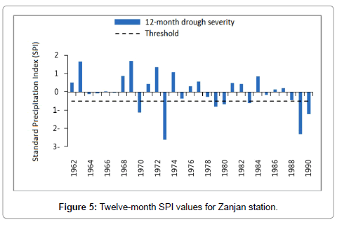
Figure 5: Twelve-month SPI values for Zanjan station.
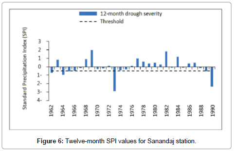
Figure 6: Twelve-month SPI values for Sanandaj station.
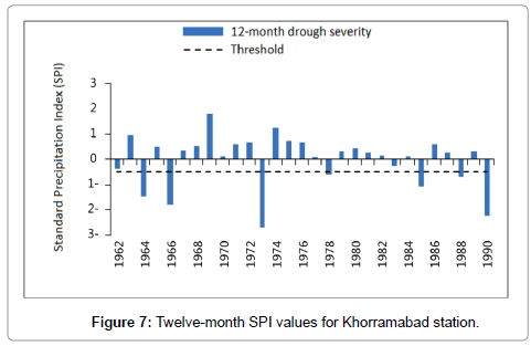
Figure 7: Twelve-month SPI values for Khorramabad station.
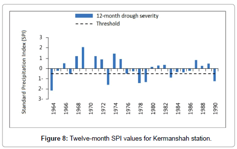
Figure 8: Twelve-month SPI values for Kermanshah station.
Estimation of drought quantity at different return periods for near future (2011-2030)
To estimate the return periods of drought during 2011-2030 (near future), the precipitation data of the desired period should be downscaled. Precipitation downscaling was performed with LARS-WG using daily observation data of the period of 1961-1990, including minimum and maximum temperature, daily rainfall, and sunshine hours. To provide future scenarios of temperature and precipitation by LARS-WG, the climatic parameters of precipitation of the stations were first calculated using the relevant function in LARS-WG using observation data of 30 years in the stations. Then to generate data for 100 years, the model was implemented according to the parameters obtained from each station. The operation was replicated several times by changing the random number aiming at obtaining statistically significant results. To evaluate the capabilities of LARS-WG in simulation of weather data, one can compare the means and variances of climate variables using T and F tests [12]. The results of t-test for the stations indicated that no significant difference existed between the mean of simulated precipitation and its actual amount at the baseline period at the significance level of 0.05. The correlation and bias coefficients and the mean absolute error in monthly series of observation and simulated data were also calculated for each station. The results are shown in Table 3. The results showed that the monthly mean precipitations were well simulated in stations of Ilam, Kermanshah, Hamedan and Sanandaj. In Zanjan, Sanandaj, and Kermanshah stations, precipitation was underestimated in some months. However, the correlation coefficient indicates well simulation of correlation between the two series of observation and simulation. The mean monthly precipitation and its standard deviations for two stations (i.e. Khoramabad and Hamedan) are shown in Figure 9. As the results indicated the best estimates of changes trend and amount were simulated in the two stations of Ilam and Zanjan. The standard deviation was underestimated for all the stations except for Ilam and Zanjanin for most months. Semenove [12] reported that this model tends to underestimate the variance in monthly means of some weather variables such as precipitation. LARS-WG was implemented for the period of 2011-2030 using the outputs of HadCM3 general circulation climate model under three scenarios of A1B, A2, and B1 by producing 80 years of daily precipitation data through calibration of LARS-WG and relying on its ability to simulate the optimal set of data for the stations (Tables 4 and 5). The Percentage Difference of precipitation in the future compared to the baseline was calculated by the following equation.
 (2)
(2)
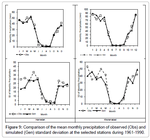
Figure 9: Comparison of the mean monthly precipitation of observed (Obs) and simulated (Gen) standard deviation at the selected stations during 1961-1990.
| Station | BIAS | MAE | Correlation |
|---|---|---|---|
| Ilam | 0.9 | 3.5 | 0.99 |
| Khorramabad | 0.3 | 5.8 | 0.97 |
| Zanjan | 0.4 | 3.5 | 0.97 |
| Sanandaj | -1.3 | 2.9 | 0.99 |
| Kermanshah | 0.4 | 4.2 | 0.98 |
| Hamedan | -0.3 | 2.8 | 0.98 |
Table 3: Comparison of the observed and simulated precipitation by LARS-WG5 in the period of 1961-1990.
| Station | Mean annual precipitation | |
|---|---|---|
| Observation period | Model baseline period | |
| Ilam | 616 | 592.8 |
| Khorramabad | 509 | 498.9 |
| Zanjan | 313.1 | 310 |
| Sanandaj | 458.4 | 420 |
| Kermanshah | 445.1 | 451 |
| Hamedan | 317.7 | 314.9 |
Table 4: Mean annual precipitation (mm) during the observed and simulated periods.
| Station | Change relative to the baseline period (%) | ||
|---|---|---|---|
| A2 scenario | A1B scenario | B1 scenario | |
| Ilam | 10.6 | 3.5 | 17.2 |
| Khorramabad | 3.8 | 3.6 | 12.9 |
| Zanjan | -1.2 | 2.6 | 3.8 |
| Sanandaj | 5.4 | 10 | 13.8 |
| Kermanshah | 13.1 | 12.4 | 28.3 |
| Hamedan | 5.2 | 1.7 | 13.5 |
Table 5: The percentage difference between precipitation during 2030-2011 and the baseline period of 1961-1990.
The spatial patterns of the changes percentage in the downscaled mean annual precipitation under the three scenarios is given in Figure 10. As can be seen, among the stations studied, an insignificant reduction in precipitation is observed in Zanjan station under the A2 scenario as 1.2%; it can be concluded that precipitation under this scenario will not change during 2011-2030. As the synthetic weather is used as the inputs for SPI software, the performance of LARS-WG should be tested by comparing the calculated values of SPI using observed and synthetic daily weather [12]. For this propose, SPI values were calculated using the amounts of precipitation during the observed and model simulated (baseline) periods. The values of SPI28-30]. The model’s performance criteria, i.e. the coefficient of determination and the slope of the fitted regression line on the intensities of drought, were compared in different return periods during observation and simulation. The results are given in Figure 11. The calculated coefficient of determination between the intensities of observed and simulated drought of the studied stations varied from 96% to 99% (the highest and lowest intensities were seen in Ilam and Khorramabad stations, respectively); these values indicate the optimum performance of the model. Given the significance of regression slope (at the level of α=0.05) and proper distribution of data within the 95% confidence interval around the mean (Figure 11), the model estimated drought severity of return periods with a desirable capability, so that they do not differ significantly with each other at the confidence level of 95%. The graphs plotted for Khorramabad and Hamedan are given as an example in Figure 11. Given the ability of the model to estimate the severity of drought in different return periods, the values of 12-month SPI were calculated using downscaled precipitation data of HadCM3 for the period of 2011-2030. Then the severities of droughts in the return periods of 2, 5, 10, 20, 25, 50, and 100 years were obtained through fitting of the proper distribution for values of less than -1 in this index; the results are given in Table 6. The results showed that the stations of Ilam, Kermanshah, Sanandaj, and Zanjan had a higher drought severity in return periods of 2, 5, and 10 years than the baseline period. For the return period of 50 years, the severity of drought was estimated more than the baseline period in three stations of Kermanshah, Zanjan, and Khorramabad, in order of magnitude [31-33]. The difference was more significant in Kermanshah station. However, the possibility of drought in this return period was less severe in Sanandaj and Ilam stations. The severity of drought for return period of 100 years was higher than the baseline in Kermanshah, Khorramabad, and Zanjan stations for near future.
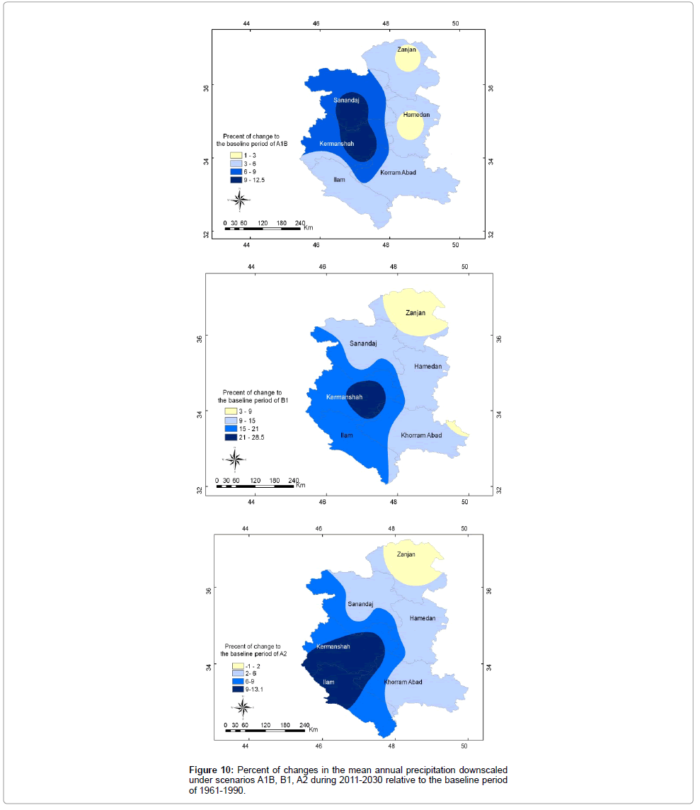
Figure 10: Percent of changes in the mean annual precipitation downscaled under scenarios A1B, B1, A2 during 2011-2030 relative to the baseline period of 1961-1990.
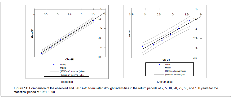
Figure 11: Comparison of the observed and LARS-WG-simulated drought intensities in the return periods of 2, 5, 10, 20, 25, 50, and 100 years for the statistical period of 1961-1990.
| ReturnPeriod | Ilam | Hamedan | Kermanshah | ||||||
|---|---|---|---|---|---|---|---|---|---|
| Baseline period | Model’s baseline period | Near future | Baseline period | Model’s baseline period | Near future | Baseline period | Model’s baseline period | Near future | |
| 2 | -1.4 | -1.5 | -1.4 | -1.5 | -1.5 | -1.6 | -1.5 | -1.4 | -1.7 |
| 5 | -1.8 | -1.8 | -1.7 | -2.1 | -2.0 | ?? | -1.7 | -1.9 | -2.5 |
| 10 | -2.0 | -2.1 | -2.0 | -2.5 | -2.4 | -2.3 | -1.9 | -2.2 | -3.0 |
| 20 | -2.3 | -2.3 | -2.3 | -2.9 | -2.8 | -2.6 | -2.0 | -2.5 | -3.5 |
| 25 | -2.4 | -2.4 | -2.4 | -3.0 | -3.0 | -2.7 | -2.0 | -2.6 | -3.7 |
| 50 | -2.6 | -2.6 | -2.6 | -3.3 | -3.5 | -2.9 | -2.1 | -2.9 | -4.2 |
| 100 | -2.9 | -2.8 | -2.9 | -3.7 | -4.2 | -3.3 | -2.2 | -3.2 | 4.7 |
| ReturnPeriod | Khorramabad | Sanandaj | Zanjan | ||||||
| Baseline period | Model’s baseline period | Near future | Baseline period | Model’s baseline period | Near future | Baseline period | Model’s baseline period | Near future | |
| 2 | -1.6 | -1.4 | -1.4 | -1.5 | -0.6 | -1.5 | -1.7 | -0.6 | -1.4 |
| 5 | -2.0 | -1.8 | -1.7 | -1.9 | -1.2 | -1.9 | -2.1 | -1.1 | -1.9 |
| 10 | -2.3 | -2.1 | -2.0 | -2.2 | -1.7 | -2.2 | -2.3 | -1.6 | -2.2 |
| 20 | -2.5 | -2.4 | -2.3 | -2.5 | -2.3 | -2.4 | -2.5 | -2.0 | -2.6 |
| 25 | -2.6 | -2.4 | -2.4 | -2.6 | -2.4 | -2.5 | -2.6 | -2.2 | -2.7 |
| 50 | -2.8 | -2.7 | -2.8 | -2.8 | -3.0 | -2.8 | -2.8 | -2.6 | -3.0 |
| 100 | -2.9 | -3.1 | -3.2 | -3.1 | -3.6 | -3.1 | -2.9 | -3.1 | -3.4 |
Table 6: The values of 12-month drought in different return periods.
Conclusion
One of the challenges facing Iran in the coming years is the water crisis which necessitates providing a prospect for future state of the climate variables such as precipitation and temperature. This is currently performed through the most reliable tool for prediction i.e. Climate models. This study was carried out during the period of 2011- 2030 in selected stations in western Iran including Ilam, Hamedan, Kermanshah, Khorramabad, Sanandaj, and Zanjan aiming at predicting drought conditions. To this end, the precipitation scenarios of HadCM3 model were applied, but since the output of these models are presented on a large scale (about 300 km2 in the model), the climatic variables obtained from these models need to be downscaled for impact assessment at station scale. Among different methods of downscaling (i.e. Statistical and dynamical methods) [34-38], the model of LARSWG was used in this study. The climatic variables were extracted at first using precipitation data observed at each station during 1961- 1990. The model was then calibrated and its capability for generating precipitation time series was ensured through comparison of the data simulated with precipitation amounts at the confidence level of 95%. The precipitation variable was downscaled using the outputs of HadCM3 general circulation model under three scenarios of A1B, A2, and B1 for near future (2011-2030). The Standardized Precipitation Index (SPI) was used to evaluate drought. The results showed that under the three scenarios, the amount of precipitation will not change significantly compared to the baseline in near future (2020s). The highest change percentage with an increase of 28% was observed in Kermanshah station at the B1 scenario. The return periods of 2, 5, 10, 20, 25, 50, and 100- year with a 12-month drought severity was then calculated. The results showed that in near future, drought in longer return period (100-year) will be more severe in the stations of Kermanshah, Khorramabad, and Zanjan compared to the baseline period. The predictions resulted from downscaling of climate models outputs were somewhat uncertain due to the structure of general circulation models, downscaling methods, observed data, etc., but since the climate models are the most reliable means of production of climate scenarios, it is essential for managers and decision-makers in various sectors of water resources, agriculture, etc. to take into account the results of such research to allow long-term planning of water resources in this region.
Suggestions
Given the other downscaling methods and output of general circulation models under different scenarios of emissions, and aiming at reducing uncertainty in the results, it is recommended to calculate the Standardized Precipitation Index using the output of these models and other statistical downscaling methods such as SDSM, ASD, etc., or dynamic downscaling methods and to compare the results and, if possible, to report the average results as more definite prediction of this index. Regarding the prediction of this index for future periods, it also suggested to provide a prospect of this index for the end of the century.
References
- Burke E, Brown JSJ (2010) Regional drought over the UK and changes in the future. J Hydrol 394: 471-485.
- Intergovernmental Panel on Climate Change (2010) Meeting Report, IPCC Expert Meeting on Assessing and Combining Multi Model Climate Projections, National Center for Atmospheric Research, Boulder, Colorado. USA.
- Gonza´lez J, Valde´s JB (2006) New drought frequency index: Definition and comparative performance analysis. Water Resources Res 42: W11421.
- Heim RR (2002) A review of twentieth-century drought indices used in the United States. BulletinAm Meteorol Soc 83: 1149-1165.
- Keyantash JA and. Dracup JA (2002) The quantification of drought: An evaluation of drought indices. Bull Amer Meteor Soc 83: 1167-1180.
- Palmer WC (1965) Meteorological Drought. Research Paper, US Weather Bureau, Washington, DC, 45:58-52.
- McKee TB, Doesken NJ, Kliest J (1993) The Relationship of Drought Frequency and Duration to Time Scales. Proceedings of the 8th Conference of Applied Climatology. 17-22 January. Anaheim. CA. American Meteorological Society. Boston MA 179-184.
- Massah AR, Sadat AP (2008) The importance of global climate change and its impact on different systems. Technical workshop on the impact of climate change on water resources 13: 41-45.
- Semenov MA, Stratonovitch P (2010) Use of Multi-model Ensembles from Global Climate Models for Assessment of Climate Change Impacts. Climate Res 4: 1-14.
- Jiang Z, Song J, Li L, Chen W, Wang Z, WangJ (2012) Extreme climate events in China: IPCC-AR4 model Evaluation and projection. Climatic Change 11: 385-401.
- Sillmann J, Roeckner E (2008) Indices for extreme events in projections of anthropogenic. Climate Change 86: 83-104.
- Semenov M (2008) Simulation of extreme weather events by a stochastic weather generator. Climate Res 35: 203-212.
- Golmohammadi M, MaasahBavani AR (2011) Evaluation of drought severity and return in future periods in Gharehsou basin under climate changes. JWater and Soil 2: 25-28.
- LashniZand M, Telvari AR (2004) Climatic drought and the possibility of its prediction in six basins in western and northwestern Iran. Geographical Res 72: 11-23.
- Razii T, Shokoohi AR, Saghafian B (2003) Prediction of severity, persistence, and frequency of droughts using probabilistic methods and time series; case study, SistanBaluchestan Province. Desert Magazine 8: 24-41.
- Nasri M, Sarhaddi A, Moddaress R (2013) Analyses of probability distribution function of intensity and duration to zone drought in central Iran. Watershed Res 91: 34-51.
- Lou AM (2011) Analysis of intensity-duration and frequency of droughts in Ahwaz using the Standardized Precipitation Index, The Fourth Conference on Management of Water Resources in Iran. Amirkabir University of Technology, Tehran.
- McKee TB, Doesken NJ, Kliest J (1995) Drought Monitoring with Multiple Time Scales. In Prox, 9th Conf. on Applied Climatology, January 17-22, American Metorology Society, Massachustts: 179-184.
- Guttman NB (1998) Comparing the Palmer Drought Index and the Standardized Precipitation Index. JAWRA J American Water Resources Association 34: 113-121.
- Szinell CS, Bussay A, Szentimrey T (1998) Drought tendencies in Hungary. Int J Climatol 18: 1479-1491.
- Hayes MJ, Svobada MD, Wilhite DA, Vanyarkho OV (1999) Monitoring 1996 Drought Using the Standardized Precipitation Index. Bulletin Am Meteorol Soc 80: 50-69.
- McEvoy D, Huntington J, Abatzoglou, JT, Edwards LM (2012)An evaluation of multi-scalar drought indices in Nevada and Eastern California. Earth Interact 16: 1-18.
- Vicente-Serrano S, BeguerÃa S, Lorenzo-Lacruz J, camarero J, López-Moreno J et al. (2012) Performance of drought indices for ecological, agricultural and hydrological applications. Earth Interact, 16: 1-27.
- Hayes MJ (2002) When Is Drought? Drought Indices. Climate Impacts Specialist. National Drought Mitigation Center.
- Gordon C, Cooper C, Senior CA, Banks H, Gregory JM et al. (2000) The simulation of SST, sea ice extents and ocean heat transports in a version of the Hadley Centre coupled model without flux adjustments. Climate Dynamics 16: 147-168.
- Pope VD, Gallani, ML, Rowntree PR, Stratton RA (2000) The impact of new physical parameterizations in the Hadley Centre climate model - HadAM3. Climate Dynamics 16: 123-146.
- Semenov MA and Brooks RJ (1999) Spatial Interpolation of the LARS-WG Stochastic Weather Generator in Great Britain. Climate Res 11: 137-148.
- AsakerehH (2010) Analysis of changes in extreme precipitation in Zanjan. J Climate Research, first year 1:13-33.
- Askari A, Rahim Zadeh F (2006) Study of the variability of precipitation in recent decades in Iran. Geographical Res 58:12-29.
- Burke E, Perry J, Brown RHJ, S.J (2010) An extreme value analysis of UK drought and projections of change in the future. J Hydrol 388: 131-143.
- Hessami M, Gachon P, Quarda TBMJ, St-HailaireA(2008) Automated regression-based statistical downscaling tool. Environ Model Software 23: 813-834.
- Kiktev D, Sexton DMH, Alexander L, Folland CK (2003) Comparison of Modeled and Observed Trends in Indices of Daily Climate Extremes. J Climate 16:3560-3571.
- Masoodian O (2008) Identification of synoptic conditions associated with super-heavy precipitation in Iran. The third Conference on Management of Water Resources in Iran. University of Tabriz 43:13-18.
- Rahim ZF(2005) Changes in extreme precipitation amounts in Iran. Nivar 58:16-26.
- Semenov MA and Barrow EM (2002) LARS-WG a Stochastic Weather Generator for Use in Climate Impact Studies. User's Manual 30:15-21.
- Szalai S, Szinell CS (2000) Comparison of Two Drought Indices for Drought Monitoring in Hungary - A Case Study, Drought and Drought Mitigation in Europe. Advances in Natural and Technol Hazards Res 14: 161-166.
- Wilby RL, Dawson CW, Barrow EM (2001)a decision support tool for the assessment of regional climate change impacts. Journal of Environmental Modeling and Software 17: 147-159.
- World Meteorological Organization (2011) Weather extremes in a changing climate: hindsight on foresight.
Citation: Fattahi E, Habibi M, Kouhi M (2015) Climate Change Impact on Drought Intensity and Duration in West of Iran. J Earth Sci Clim Change. 6: 319. DOI: 10.4172/2157-7617.1000319
Copyright: © 2015 Fattahi E, et al. This is an open-access article distributed under the terms of the Creative Commons Attribution License, which permits unrestricted use, distribution, and reproduction in any medium, provided the original author and source are credited.
Select your language of interest to view the total content in your interested language
Share This Article
Recommended Journals
Open Access Journals
Article Tools
Article Usage
- Total views: 15105
- [From(publication date): 12-2015 - Aug 19, 2025]
- Breakdown by view type
- HTML page views: 13670
- PDF downloads: 1435