Climate Change Observed over the Indo-Gangetic Basin
Received: 26-Mar-2015 / Accepted Date: 06-Apr-2015 / Published Date: 16-Apr-2015 DOI: 10.4172/2157-7617.1000271
Abstract
We combine the seasonal mean precipitation and temperature from different datasets into a Bayesian framework using Multi-variable Bayesian Merging (MBaM) algorithm to draw a unified conclusion about their trend over the Indo-Gangetic Basin (IGB). The time series produced by the Bayesian method is combined into a Multi-variable Trend Principal Component (MTPC) setup to derive the equivalent climate change signals. These signals are then used to estimate the importance of different regional and global drivers influencing the climate change over the IGB. We show that the climate change over the IGB during pre-monsoon and monsoon seasons is very significant, during post-monsoon is less significant, and during winter season there is no indication of significant climate change. Global teleconnections are shown to have very little correlation to the climate change signal (e.g. RNino3=0.06∼0.21). On the other hand, the concentrations of greenhouse gases are found to exhibit very strong correlation (e.g RCO2 =0.94∼0.99) to the climate change signal, indicating their importance as drivers of the climate change over the IGB.
Keywords: Geographical variations; Bayesian framework; Global teleconnections
9132Introduction
Indo-Gangetic Basin (IGB) is the principal source of food and livelihood security for billions of people of India as well as south Asia [1]. Studies analyzing the behavior of water resources under climate change indicate significant impact on the mean annual discharge, which is governed by the changes in the intensity and frequency of precipitation distributions [2,3]. Changes in reservoir storage due to modest change in natural inflow have the ability to potentially change the energy production, flood generation, and control measure [4]. Several studies in the recent past have analyzed the climate change over the IGB [5-8]. However, there is a lack of general agreement about the magnitude, and even direction, of trends in rainfall [5,6,9-20] as well as temperature [5,7,8,10,13,21-24]. This lack of agreement may be due to various factors, e.g. exact extent of study domain (for spatial averaging), analysis method (parametric or non-parametric), and source of the gridded data. Climate is a very complex and nonlinear system consisting of a wide spectrum of variabilities within its physio-dynamical process. The simplest among them is the linear trend. Considering the entire study domain as a single entity, we can explore the mean variable trend over the region. However, when we extract a single trend response (mean response) for a region we lose the information of the geographical variation of the trend. Furthermore, given the complexity of the climate system, it may be possible that a single response is not enough to explain the total trend variation.
In this study, we analyze the precipitation data from APHRODITE, Climatic Research Unit (CRU), Global Precipitation Climatology Project (GPCC), India Meteorological Department (IMD), Precipitation Reconstruction over Land (PREC/L) and University of Delaware (UDEL), and temperature data from APHRODITE, CRU and UDEL to show that the spatial trends are strongly heterogeneous among different datasets. We estimate a unified trend of seasonal mean precipitation and temperature from previously mentioned datasets by merging them into a Bayesian framework. The grid points are assumed to be statistically homogeneous to allow us to fit data from all the datasets and grid points into a single statistical framework. We expect that this will result in a more precise estimation of different parameters than the case where each grid point is treated separately. This Multi variable Bayesian Merging (MBaM) formulation is motivated from the work of Tebaldi et al. [25] and Tebaldi et al. [26]. A major assumption of this technique is the interpretation of a dataset as a sample of the underlying climate space. Empirical Orthogonal Function (EOF) analysis derives the linear combination of input spatio-temporal variables in such a way that it maximizes their variance within an orthogonality constraint. Hannachi [27] has proposed an alternative formulation of EOF, which maximizes the trend within the climatic variable, called Trend Principal Component Analysis (TPCA). In the present work, we extend this Trend EOF method in our formulation. Temperature and rainfall, due to their close correlation with other important variables and easy availability of observations, are treated as a proxy for climatic system. Any method which combines the climatic information from these variables to an equivalent climate change signal will be very useful for the climate change studies over a geographical region. We combine the time series produced by the Bayesian method into a Multi-variable Trend Principal Component Analysis (MTPCA) setup to derive the equivalent trend principal components. These MTPCs, if significant, can be taken as the equivalent climate change signal. We use the equivalent climate change signal from MTPCA as a tool to find the relative importance of different drivers in inducing the observed climate change.
The main problems faced by any study on the climate change are: 1) finding the underlying trend from the inter contradictory datasets when actual climate characteristics are unknown, 2) defining a climate change metric based on which the magnitude of the change can be quantified, and 3) finding a set of governing factors which drive the climate change over that region. Our objective through this paper is to address these issues in the IGB geographic perspective. As studies addressing these basic problems are very scarce, we have developed a novel framework to address the above mentioned issues. We propose MBaM framework to combine various datasets to extract underlying climatic signal of any meteorological variable. We formulate MTPCA to quantify the climate change, and to extract an equivalent climate change signal from the various datasets mentioned earlier. Finally, with the help of the climate change signal and correlation analysis, we examine the importance of different global or anthropogenic drivers to the climate change over the IGB. Our novel methodology provides useful insight into the characteristics of the climate change over the IGB, and examines the possible drivers for the same.
Study Area, Datasets and Methodology
The IGB has an aerial coverage of 70,00,000 km2 and supports a population of 1 billion [28]. Considering this huge population (1/7th of total global population) the possibility of climate change over this region has a huge socio-economic implication. Figure 1 shows the location and coverage of the IGB (green shaded). We delineate the weather pattern over the IGB into four seasons, viz., winter (Jan-Feb), pre-monsoon (March-May), monsoon (Jun-Sept) and post-monsoon (Oct-Dec). The prominent meteorological phenomenon during winter is fog and during pre-monsoon is dust storm [29]. Most of the rainfall over IGB is concentrated during monsoon period [30]. Assessment of the climatic state of a region requires long-term information about the prevailing climatic conditions over that region. To create a long-term environmental database, several efforts have been made which led to the generation of extensive databases [31-36]. The datasets used in this study are examples of observational databases e.g. APHRODITE [37,38], CRU [39], GPCC [40], PREC/L [41], UDEL [42] and IMD [43]. We use the 0.5◦×0.5◦ resolution precipitation data from these datasets. However, temperature data are obtained from APHRODITE, CRU and UDEL because they are available from only these sources. From 1971 to 2005 is chosen as the study period for trend analysis.
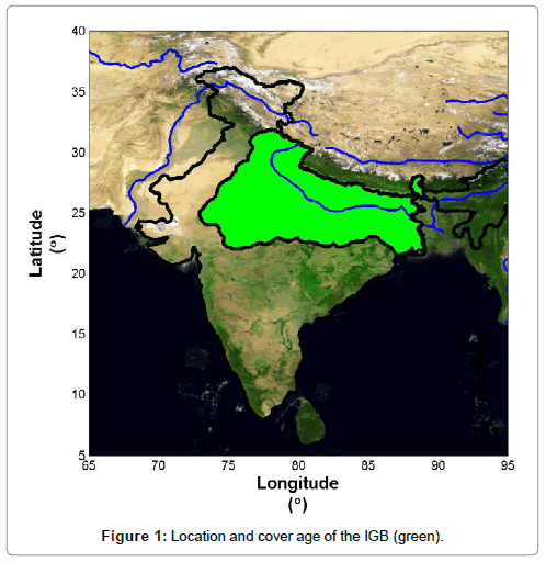
Figure 1: Location and cover age of the IGB (green).
We assume normal (N) distribution of the climate variable (precipitation or temperature) Xitl, as
 (1)
(1)
where the indices denote the grid points (i), time (t) and dataset (l). ai and bi signify the intercept and trend respectively specified at the grid point i. λi and λl are climatic precisions at individual grid point and dataset, respectively.
The assumption of normality of climatic variables, specifically for temperature, is somewhat restrictive. However, this assumption makes all the statistical features of climatic variable, viz. mean along with its trend and variances, readily identifiable. Also, this assumption of normality is also supported by the Kolmogorov-Smirnov test (in supplementary material). Equation 1 signifies that there is a linear trend for climatic variable for each grid point with intercept ai and slope bi.
The assumption that the overall precision can be factorized into two precision parameters, λi and λl, (though somewhat restrictive), simplifies the parameter estimation and enables us to estimate the individual precision parameters more precisely. This ultimately results in narrower posterior distributions. Moreover, it also provides a means of comparing the accuracy of different observational datasets. We use the Gibbs sampler to iteratively simulate the samples of the posterior distribution from the sequence of conditional distributions. We discarded the first 5000 samples in the Markov Chain Monte Carlo (MCMC) sampling as “burn in” and uniformly “sampled without replacement” 1000 samples from the latter 15,000 values after 20,000 iterations. Detailed discussion of the model is presented in the supplementary part of this paper.
The atmospheric fields like precipitation and temperature are closely related and it may be prudent to address their trends together. We extend the method given by Hannachi [27] to use the inverse rank computed from multiple variables and get a trend Principal Component (PC) which maximizes the total monotonicity considering all the variables and grid points.
Let  , Where
  denotes the data matrix of climatic variables time t=1, · · · , nt at grid points i=1, · · · , ni for number of variables v=1, · · · , nv. MTPCA uses a new matrix Q=q1, q2,··· , qni×nv of time positions of the sorted data (the inverseranks of the data). To correct the non-uniform data distribution on the geographic grid we weighted this inverse rank Q with the corresponding latitude.
Multi variable Trend Empirical Orthogonal Function is given by the Eigen vectors of the co-variance matrix  , where
  is an identity matrix and
  is a vector of ones. If the Eigen vectors of the co-variance matrix are v, then the Trend principal components (PC time series) on the physical space are given by TPC=Zv, where
  is the standard score of the data matrix.
The relative magnitude of the Eigen values represents the extent of monotonicity explained by the corresponding Eigen vectors, and the vector with highest Eigen value gives the maximum mono- tonic trend. If the distribution or Highest Posterior Density Confidence Interval (HPDCI) of an Eigen value does not overlap others at a certain credible level, then it implies that the Eigen value as well as the corresponding Eigen vector is significant at that credible level. We generated a set of samples (1000) from the posterior distribution of rainfall and temperature after omitting the precision factor of the dataset (λl), performed Eigen analysis for each of these sample streams, and generated a distribution of Eigen value spectrum. We consider the Eigen vectors corresponding to the significant Eigen values as climate change signal for the analysis period.
Correlation between the equivalent climate change signals to the time series equivalent of any climatic driver signifies the dependence of the climate change on that driver. We test the correlation along with the significance test using the 1000 samples of the climate change signal, describing the uncertainties of the climate change. The significance test is further discussed in the supplementary section of this paper.
Results
We estimate the mean trend of all the grid points and test the nonzero trend alternate hypothesis using HPDCI at 90% credible level. The grid points where the test rejects the zero trend null hypotheses are shown in the Figures 2 and 3 by asterisk (*) marks.
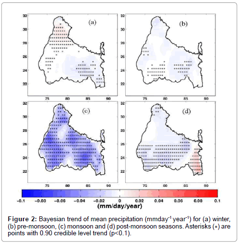
Figure 2: Bayesian trend of mean precipitation (mmday-1 year-1) for (a) winter, (b) pre-monsoon, (c) monsoon and (d) post-monsoon seasons. Asterisks (∗) are points with 0.90 credible level trend (p<0.1).
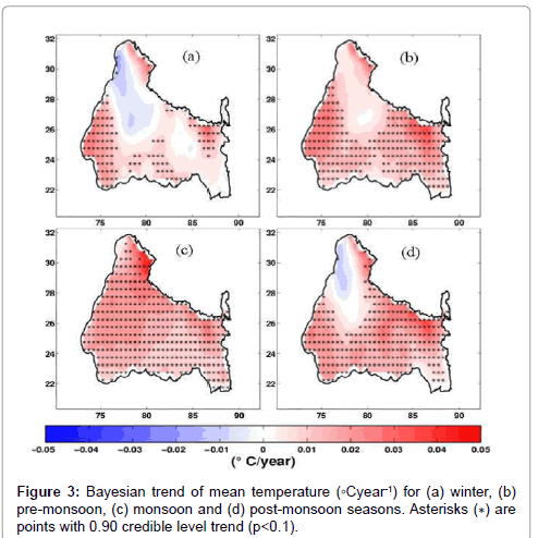
Figure 3: Bayesian trend of mean temperature (◦Cyear-1) for (a) winter, (b) pre-monsoon, (c) monsoon and (d) post-monsoon seasons. Asterisks (∗) are points with 0.90 credible level trend (p<0.1).
Figure 2 shows the spatial distribution of the trend of precipitation for different seasons. Trends in winter (Figure 2a) show a prominent bi-modal structure. The south eastern part of the basin shows prominent decreasing trend (∼-0.02 mm day-1year-1), and the north western part shows prominent increasing trend (∼0.02 mm day-1 year-1). Central IGB during winter is completely void of any trends. This trend-less characteristics of rainfall over central IGB, which during this season has more amount of rain (3 ∼ 4 mm day-1) than other part of IGB, indicates the stable behavior of climate during this season. This structure indicates the possible effects of orography [44] in the northern part and effect of the sea [45] in the south eastern part. Trend structure during pre-monsoon (Figure 2b) seasons is not coherent. Very few grid points in the southern part of IGB show significant trends (∼-0.01 mm day-1year-1). Most of the northern and central IGB are completely void of any trend during pre-monsoon season. The monsoon (Figure 2c) season shows a strong decreasing trend for almost all the grid points (-0.02 ∼ -0.1 mm day-1year-1). There are two spatial modes,: eastern and western, of these decreasing trends with a north-south discontinuity at the central IGB. There is a pocket of increasing trend (-1year-1), though not significant, at the middle Bengal, at the eastern part of the IGB. The magnitude of the trends is strongest in this season which is due to the fact that most of the rainfall over IGB is concentrated within monsoon season, thus the consistent drying is also the strongest. These reductions in rainfall received by the IGB during the monsoon period have great implication on the Agriculture and hydro-energy production as most of the rainfall over this region is received during the monsoon season. Post-monsoon (Figure 2d) season shows a de- creasing trend in the central IGB (∼- 0.02 mm day-1year-1), but at the south-eastern part there is a significant increasing trend (∼0.03 mm day-1year-1), and the northern portion does not show any significant trend. The sharp spatial change of increasing to decreasing trend indicates probable land-sea interaction in the south eastern part of IGB.
Figure 3 shows the spatial distribution of the trend of temperature for the different seasons. The significant increasing trend is quite consistent in all the seasons. During winter (Figure 3a), the south western and north eastern parts of the IGB show significant warming (0.02° ∼ 0.04°C year-1). The north western part of the IGB has a cold mode (∼ –0.01°C year-1), which de- spite its lesser statistical significance, indicates the possible effects of cold westerly during this season. During pre-monsoon (Figure 3b), apart from north eastern part of the IGB (∼ 0.01°C year-1), the entire basin shows a consistent significant warming trend (0.02° ∼ 0.05°C year-1).
We speculate, orographic effects of Himalaya are affecting the trend-less grid points at the north. During monsoon season (Figure 3c), the entire IGB shows consistent significant increasing trend (0.02° ∼ 0.04°C year-1). Like winter, post-monsoon (Figure 3d) has a similar “dual modal” structure. Apart from a pocket at the north east of the IGB (∼ –0.01°C year-1) the entire IGB shows significant increasing trend (0.02° ∼ 0.04°C year-1). The north eastern points show decreasing but not significant trend. We speculate, the effect of cold western disturbance is inducing this cold pocket [46].
Figures 4a-4d shows the Eigen value spectrum and their credible interval for different seasons. The circle denotes the mean for the distribution of Eigen value and the bar denotes the corresponding spread at 0.90 credible level (p<0.1). For winter (Figure 4a), the 1st Eigen value is not significantly different from the 2nd Eigen value. For pre-monsoon (Figure 4b), and monsoon (Figure 4c), the 1st Eigen value is significantly different from the 2nd Eigen value. For post-monsoon (Figure 4d), the Eigen values are non-overlapping at lower (∼85%) credible level. These indicate that the IGB does not show a climate change during winter but during pre-monsoon and monsoon, the climate change is significant. During post-monsoon some indication of the climate change is present but with lower confidence (p<0.15).
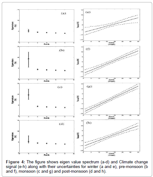
Figure 4: The figure shows eigen value spectrum (a-d) and Climate change signal (e-h) along with their uncertainties for winter (a and e), pre-monsoon (b and f), monsoon (c and g) and post-monsoon (d and h).
Figures 4e-4h show the trend principal components along with their uncertainty band, which represents the equivalent climate change signal, for different seasons. The solid line denotes the mean of the principal component distribution and the dashed lines denote its spread at 0.90 credible level (p<0.1). For winter (Figure 4e), the lower and upper ends of the signal show considerable amount of uncertainties, which in turn makes the trend in the climate change signal negligible. For pre-monsoon (Figure 4f), monsoon (Figure 4g), and post-monsoon (Figure 4h), the signal shows a sharp linear change which indicates that the climate change over the IGB during those seasons is statistically significant.
Teleconnections are well known markers for synoptic scale dependence on regional climatic systems [47]. Sea-surface temperature or sea level pressure from some region can dynamically alter the climate over another distant region [48]. Tele-connection in- dices are the time series representations of the teleconnections. In Table 1, we use the correlation between the teleconnection index and the equivalent climate change signal to measure the dependence of the climate change over the IGB on the synoptic scale drivers. The significant correlations are marked with bold font. The east-pacific north-pacific oscillation index during pre-monsoon season (R=0.51), nino 4 index during monsoon season (R=0.47), and western hemisphere warm pool index during monsoon (R=0.68) and post-monsoon seasons (R=0.58), are significantly correlated to the climate change signals. The tropical northern Atlantic index is significantly correlated (R=0.39 ∼ 0.64) to the climate change signals during all the seasons. Despite these significant correlations, considering the overall correlation values we find that the climate change signal has little or no dependence on most of the global teleconnection indices.
| Teleconnection/Seasons | Winter | Pre-monsoon | Monsoon | Post-monsoon |
|---|---|---|---|---|
| East PacificNorth PacificOscn | 0.11 | 0.51 | -0.30 | -0.02 |
| Nino1+2 | 0.21 | 0.13 | 0.06 | 0.15 |
| Nino3 | 0.15 | 0.29 | 0.19 | 0.09 |
| Nino3.4 | 0.15 | 0.30 | 0.28 | 0.12 |
| Nino4 | 0.25 | 0.34 | 0.47 | 0.29 |
| NorthAtlanticOscillation | 0.33 | 0.11 | -0.21 | -0.22 |
| PacificDecadalOscillation | 0.29 | 0.37 | 0.16 | -0.04 |
| PacificNorthAmericanIndex | 0.23 | 0.00 | 0.21 | 0.18 |
| SouthernOscillationIndex | -0.11 | -0.29 | -0.19 | -0.05 |
| TropicalNorthernAtlanticIndex | 0.39 | 0.42 | 0.64 | 0.64 |
| TropicalSouthernAtlanticIndex | 0.31 | 0.32 | 0.13 | 0.27 |
| WesternHemispherewarmpool | 0.12 | 0.35 | 0.68 | 0.58 |
| WesternPacificIndex | 0.33 | -0.10 | -0.25 | -0.14 |
| IndianOceanDipole | -0.09 | -0.17 | 0.00 | 0.01 |
Table 1: Correlation between different tele-connection indices and the IGB climate change signals.
Recent studies have identified anthropogenic emissions as the major cause of the climatic trends [49], which may in turn also affect the ecosystem [50,51]. The globally averaged Green House Gases (GHGs) are an excellent representative time series for these anthropogenic GHG concentrations. In Table 2 we use the correlation between the concentration time series and the equivalent climate change signal to measure the dependence of the climate change of the IGB on the anthropogenic drivers. All the GHGs are observed to be significantly correlated to the climate change signal during all the seasons. The average strength of correlations are maximum for CO2 (R=0.94∼0.99) and N2O (R=0.94∼0.99) indicating these two as the most prominent anthropogenic drivers of the climate change. During winter, when the significant climate change is absent, the correlation of these anthropogenic drivers is the weakest.
| GHG/Seasons | Winter | Pre-monsoon | Monsoon | Post-monsoon |
|---|---|---|---|---|
| CO2 | 0.94 | 0.99 | 0.99 | 0.98 |
| N2O | 0.94 | 0.99 | 0.99 | 0.99 |
| CH4 | 0.90 | 0.95 | 0.96 | 0.95 |
| CFC11 | 0.89 | 0.94 | 0.94 | 0.93 |
| CFC12 | 0.91 | 0.96 | 0.96 | 0.95 |
Table 2: Correlation between different global GHG concentrations and the IGB climate change signals.
Summary
We have analyzed the dataset from multiple sources to show that the spatial trend characteristics vary considerably among different datasets. To address this issue we propose a Bayesian framework to get unified trends considering all those datasets. A number of samples from the equivalent dataset, after removing the effect of the individual observation dataset, are prepared using the parameters derived from the Bayesian framework. The samples from this analysis are specified into a MTPCA framework to derive the equivalent climate change signal for the IGB during different seasons. We show that the climate over the IGB is significantly (>90% confidence level) changing during pre-monsoon and monsoon seasons. During post-monsoon, the change occurs with slightly lesser significance (∼ 85% confidence level). During winter season, the indication of any climate change is absent. The equivalent climate change signal is further used to analyze the importance of different climatic drivers in inducing the climate change over the IGB. We find the global teleconnection has negligible importance in inducing the climate change. The concentrations of GHGs have very strong correlation to the climate change signal indicating their prime importance as drivers of the climate change over the IGB. These results indicate that the teleconnection indices, which may be responsible for inter annual variabilities or hydrological extremes (e.g. drought), may not play a significant role in long-term climatic trend over the IGB. On the other hand, GHG, which may not be responsible for interannual variabilities, can play an important part in the climate change process over the IGB. The novel methods formulated in this paper are not restricted to the analysis of climate over IGB, but can be used in analysis of climatic characteristics of any region. These methods will help us in understanding the climatic properties of any region and the processes which induce them.
Acknowledgements
We thank APHRODITE’s Water Resources Project members and University of East Anglia for archiving the APHRODITE and CRU data, respectively. We acknowledge NOAA for archiving the GPCC and PREC/L data. We thank IMD for providing the IMD gridded rainfall data.
References
- Paroda RS, Woodhead T, Singh RB (1994) Sustainability of rice-wheat production systems in Asia. RAPA Publication, Bangkok.
- Whitfield PH, Cannon AJ (2000) Recent variations in climate and hydrology in Canada. Canadian Water Resour J 25: 19-65.
- Muzik I (2001) Sensitivity of hydrologic systems to climate change. Canadian Water Resour J 26: 233-253.
- Xu C-Y, Singh V (2004) Review on regional water resources assessment models under stationary and changing climate. Water Resour Manage 18: 591-612.
- Pant GB, Hingane LS (1988) Climatic changes in and around the rajasthan desert during the 20th century. Int J Climatol 8: 391-401.
- Bollasina MA, Ming Y, Ramaswamy V (2011) Anthropogenic aerosols and the weakening of the south asian summer monsoon. Sci 334: 502-505.
- Hingane LS, Kumar KR, Murty VR (1985) Long-term trends of surface air temperature in India. Int J Climatol 5: 521-528.
- Subash N, Sikka AK, Mohan HSR (2010) An investigation into observational characteristics of rainfall and temperature in central northeast India- a historical perspective 1889-2008. TheorApplClimatol 103: 305-319.
- Subbaramayya I, Naidu CV (1992) Spatial variations and trends in the indian monsoon rainfall. Int J Climatol 12: 597-609.
- Kothyari UC, Singh VP (1996) Rainfall and temperature trends in India. Hydrol Process 10: 357-372.
- Mirza MQ, Warrick RA, Ericksen NJ, Kenny GJ (1998) Trends and persistence in precipitation in the Ganges, Brahmaputra and Meghna river basins. HydrolSci J 43: 845-858.
- Naidu CV, Rao BRS, Rao DVB (1999) Climatic trends and periodicities of annual rainfall over India. MeteorolAppl 6: 395-404.
- Singh N, Sontakke NA (2002) On climatic fluctuations and environmental changes of the Indo-Gangetic plains, India. Climatic Change 52: 287-313.
- Singh N, Sontakke NA, Singh HN, Pandey AK (2005) Recent trend in spatiotemporal variation of rainfall over Indian investigation into basin-scale rainfall fluctuations. IAHS Publication 296: 273-282.
- Dash SK, Jenamani RK, Kalsi SR, Panda SK (2007) Some evidence of climate change in twentieth-century India. Climatic Change 85: 299-321.
- Ramesh KV, Goswami P (2007) The shrinking Indian summer monsoon. Tech. rep., CSIR Centre for Mathematical Modelling and Computer Simulation.
- Guhathakurta P, Rajeevan M (2008) Trends in the rainfall pattern over India. Int J Climatol 28: 1453-1469.
- Ranade A, Singh N, Singh HN, Sontakke NA (2008) On variability of hydrological wet season, seasonal rainfall and rainwater potential of the river basins of India (1813-2006). J Hydrol Res Dev 23: 79-108.
- Basistha A, Arya DS, Goel NK (2009) Analysis of historical changes in rainfall in the Indian Himalayas. Int J Climatol 29: 555-572.
- Kumar V, Jain SK (2010) Trends in rainfall amount and number of rainy days in river basins of India (1951-2004). Hydrol Res 42: 290-306.
- Pant GB, Kumar KR (1996) Climates of South Asia. John Wiley, Chichester UK.
- Arora, M, Goel NK, Singh P (2005) Evaluation of temperature trends over India. HydrolSci J 50: 81-93.
- Singh P, Kumar V, Thomas T, Arora M (2008) Basin-wide assessment of temperature trends in Northwest and Central India. HydrolSci J 53: 421-433.
- Kothawale DR, Revadekar JV, Kumar KR (2010) Recent trends in pre-monsoon daily temperature extremes over India. J Earth Syst Sci 119: 51-65.
- Tebaldi C, Mearns LO, Nychka D, Smith RL (2004) Regional probabilities of precipitation change: A bayesian analysis of multimodel simulations. Geophys Res Lett 31.
- Tebaldi C, Smith RL, Nychka D, Mearns L (2005) Quantifying uncertainty in projections of regional climate change: a bayesian approach to the analysis of multimodel ensembles. J Climate 18: 1524-1540.
- Hannachi A (2007) Pattern hunting in climate: a new method for finding trends in gridded climate data. Int J Climatol 27: 1-15.
- TWF (2013) The world factbook 2013-14. Central Intelligence Agency, Washington DC.
- Kumar R, Barth MC, Pfister GG, Naja M, Brasseur GP (2014) WRF-chem simulations of a typical pre-monsoon dust storm in northern india: influences on aerosol optical properties and radiation budget. Atmos Chem Phys 14: 2431-2446.
- Krishnamurthy V, Shukla J (2007) Intraseasonal and seasonally persisting patterns of Indian monsoon rainfall. J Climate 20: 3-20.
- Juang HH, Hong HS, Kanamitsu M (1997) The NCEP regional spectral model: an update. Bull Am MeteorolSoc 78: 2125-2143.
- Gunther H, Rosenthal W, Stawarz M, Carretero JC, Gomez M, et al. (1998) The wave climate of the Northeast Atlantic over the period 19551994: the wasa wave hindcast. Global Atmos Ocean Syst 6: 121-163.
- Ebisuzaki W, Kanamitsu M, Potter J, Fiorino M (1998) An overview of reanalysis-2, Miami, Florida.
- Cox AT, Swail VR (2001) A global wave hindcast over the period 19581997: validation and climate assessment. J Geophys Res 106: 2313-2329.
- Feser F, Weisse R, Storch HV (2001) Multi-decadal atmospheric modelling for europe yields multi-purpose data. Eos Trans 82: 305-310.
- Guedes C, Carretero JC, Weisse R, Alvarez E (2002) A 40 years hindcast of wind, sea-level and waves in european waters. Proceedings of OMAE 2002: 21st International conference on offshore mechanics and arctic engineering, Oslo, Norway.
- Yatagai A, Kamiguchi K, Arakawa O, Hamada A, Yasutomi N, et al. (2012) Aphrodite: Constructing a long-term daily gridded precipitation dataset for asia based on a dense network of rain gauges. Bull Am MeteorolSoc 93: 1401-1415.
- Yasutomi N, Hamada A, Yatagai A (2011) Development of a long-term daily gridded temperature dataset and its application to rain/snow discrimination of daily precipitation. Global Environ Res 15: 165-172.
- Harris I, Jones P, Osborna T, Listera D (2013) Updated high-resolution grids of monthly climatic observations the cru ts3.10 dataset. Int J Climatol 34: 623-642.
- Schneider U, Becker A, Finger P, Christoffer AM, Ziese M, et al. (2014) GPCC’s new land surface precipitation climatology based on quality-controlled in situ data and its role in quantifying the global water cycle. Theor Appl Climatol 115: 15-40.
- Chen M, Xie P, Janowiak JE (2002) Global land precipitation: A 50-yr monthly analysis based on gauge observations. J Hydrometeor 3: 249-266.
- Legates DR, Willmott CJ (1990) Mean seasonal and spatial variability in gauge-corrected, global precipitation. Int J Climatol 10: 111-127.
- Rajeevan M, Bhate J, Kale JD, Lal B (2006) High resolution daily gridded rainfall data for the Indian region: Analysis of break and active monsoon spells. Curr Sci 91: 296-306.
- Kulkarni A, Patwardhan S, Kumar KK, Ashok K, Krishnan R (2013) Projected climate change in the Hindu Kushhimalayan region by using the high-resolution regional climate model precis. Mountain Res Develop 33: 142-151.
- Bollasina M, Nigam S (2008) Indian Ocean SST, evaporation, and precipitation during the South Asian summer monsoon in IPCC-AR4 coupled simulations. Climate Dyn 33: 1017-1032.
- Lall JS, Moddie AD (1981) The Himalaya, aspects of change. India International Centre, India.
- Wang D, Wang C, Yang X, Lu J (2005) Winter northern hemisphere surface air temperature variability associated with the arctic oscillation and North Atlantic oscillation. Geophys Res Lett 32.
- Lu R, Dong B (2005) Impact of atlantic sea surface temperature anomalies on the summer climate in the western north pacific during 19971998. J Geophys Res: Atmos 110.
- Ramaswamy V (2009) Anthropogenic climate change in Asia:Â Key challenges. Trans Am Geophys Union 90: 469-480.
- Wali M, Evrendilek F, West T, Watts S, Pant D, et al. (1999) Assessing terrestrial ecosystem sustainability: usefulness of regional carbon and nitrogen models. Nature Resour 35: 20-33.
- Evrendilek F, Berberoglu S (2008) Quantifying spatial patterns of bioclimatic zones and controls in turkey. Theor Appl Climatol 91: 35-50.
Citation: Chaudhuri C, Srivastava R, Tripathi SN, Misra A (2015) Climate Change Observed over the Indo-Gangetic Basin. J Earth Sci Clim Change 6: 271. DOI: 10.4172/2157-7617.1000271
Copyright: ©2015 Chaudhuri C, et al. This is an open-access article distributed under the terms of the Creative Commons Attribution License, which permits unrestricted use, distribution, and reproduction in any medium, provided the original author and source are credited.
Select your language of interest to view the total content in your interested language
Share This Article
Recommended Journals
Open Access Journals
Article Tools
Article Usage
- Total views: 16502
- [From(publication date): 4-2015 - Jul 01, 2025]
- Breakdown by view type
- HTML page views: 11823
- PDF downloads: 4679