Journal of Earth Science & Climatic Change
Open Access

Since the beginning of this century (2000-2016) the humanity has suffered from dozens of destructive earthquakes with magnitude over M≥6, including two catastrophic earthquakes (Sumatra 26.12.04 and Japan 11.03.11) with magnitude over M≥9. They destroyed entire settlements and infrastructure - bridges, highways, roads, flooded islands, coastal harbors and power stations. The human victims amount to several hundred thousand. Material damages are in the same order reaching billions of dollars. The earthquake history constantly proves the unpredictability of power, place and time of the next cataclysm [1-4].

According to statistics, the number of devastating earthquakes increases over the time [5], whereas the geographical distribution is (Latitude, Longitude) predominantly in the “Fire ring” - along the boundaries of the main geotectonic plates and the fault lines. The process of occurrence of the cataclysm is probable. Some earthquakes forecast researches are given in [6-13]. Teams from different countries are availing themselves of modern satellite technologies. Efforts are focused on studying changes in the ionosphere, underwater currents in the World Ocean, tides, electromagnetic emissions, thermal anomalies, etc.

In this study is presented information on the thermal anomalies (OLR) collected by the satellites during the earthquakes and from the past two years without earthquakes for the relevant geographic locations. It is known that the masses of the tectonic plates are subjected to enormous pressure and critical stresses are generated whereby positively charged particles “p-holes” are emitted. When these reach the ground, they ionize the molecules of the air and infrared rays are emitted. It is known as OLR. The satellite sensors at tens of kilometers catch the infrared radiation and keep track of it as a reflection from the Earth's surface with wavelength of 10-13 μm.

Nomenclature

- The average OLR value per day for the two years without collision is

The momentary OLR value in the course of the year with an earthquake is

Maximum and minimum value of the variation

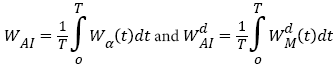
WAI - Average integral value of the over the period considered in

WAA - Average algebraic value of the

Average integral value of the over the years with earthquakes in

- Average algebraic value of the in

Times in which in The time in which the earthquake occurs in [days]. Maximum energy limit of the OLR in

The time after which the earthquake occurs in [days]

Energy assessment of the OLR signals

Figures 1a and 1b are shown examples of variations of OLR signals. One of the figures represents variations of OLR signal without any seismic phenomena for a two- year long period for the specific place on Earth with geographical coordinates – Latitude and Longitude. The other figure represents the OLR signal for the same place of the Earth with the same geographical coordinates, but for a time period of one year with occurrence of big seismic phenomena. The minimum and maximum values are as follows:

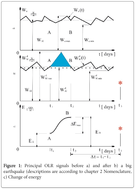
Figure 1: Principal OLR signals before a) and after b) a big earthquake (descriptions are according to chapter 2 Nomenclature, c) Change of energy

(1)

These are exhibited in the two figures.

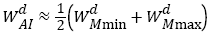
Extensive analysis (hundred occurred earthquakes with M>6) shows that the difference between the average integral OLR signal values and the arithmetical average values is less than 5%. For this reason, could be assumed that:

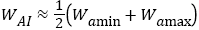and

(2)

The variation of the energy of the OLR signal in the time interval is shown in the Figure 1c where the variation is most significant. The points A and B match aligned values of:

hence (3)

The largest amount of change of energy in a year with an earthquake is determined by the expression:

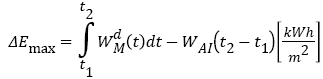(4)

The extent of variation of the radiation during the period of two years without any cataclysms is :

(5)

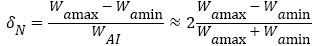
and the extent of variation of the radiation during the period with cataclysms is :

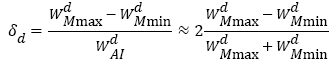(6)

which are additional criteria for earthquake forecast. On the Figures 1b and 1c with star is marked the earthquake occurrence at time point .

Comparison between NOAA 15 and NOAA 18 satellites data [3]

First the anomaly was recorded during the day of passing of “NOAA 15” satellite on August 31, 2015 (Figure 2). The anomaly started disappearing on the same day but a less intense OLR anomaly was recorded during the night of passing of the “NOAA 18” satellite on August 31, 2015 (Figure 3).

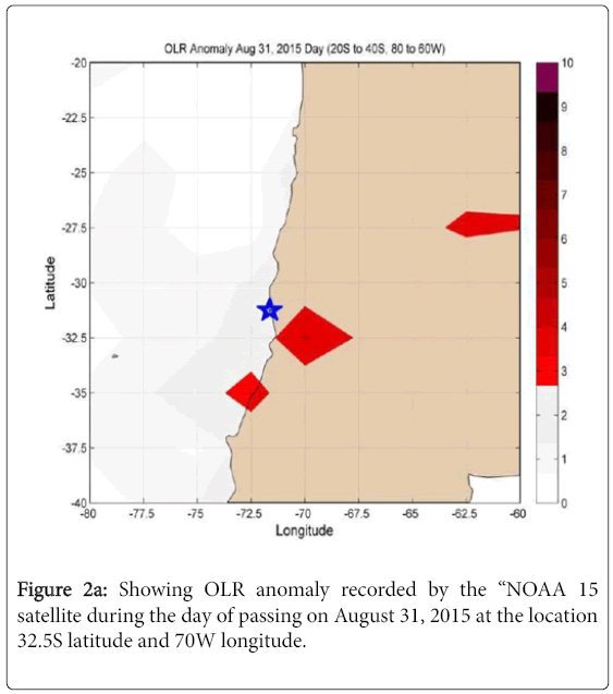
Figure 2a: Showing OLR anomaly recorded by the “NOAA 15 satellite during the day of passing on August 31, 2015 at the location 32.5S latitude and 70W longitude.

Figure 2b: Graph showing OLR scenario at the location 32.5S latitude and 70W longitude between August 15, 2015 and Sep 17, 2015.

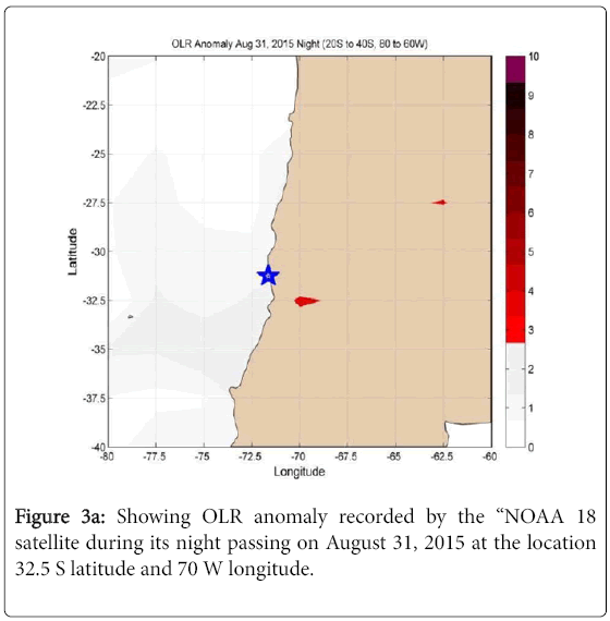
Figure 3a: Showing OLR anomaly recorded by the “NOAA 18 satellite during its night passing on August 31, 2015 at the location 32.5 S latitude and 70 W longitude.

Figure 3b: Figure shows OLR scenario at the location 32.5 S latitude and 70 W longitudes between August 15, 2015 and Sep 17, 2015.

Information is presented in Figures 2 and 3 in graphical mode from the first satellite NOAA 15 Figure 2a and the second satellite NOAA 18 Figure 3a in case of identical geographical coordinates. Two curves in the same Figure 2b and Figure 3b correspond to variations of the OLR without any earthquakes and variations of the OLR with the Chili earthquake 16.09.2015. Figure 2b and Figure 3b show clearly the anomaly and the similarity of the two figures.

The following numerical results are reached following the abovementioned methodology:

From Figure 2b, 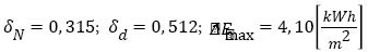(Table 1); (see the star * on Figure 1c); From Figure 3b, 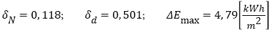(Table 1); (see the star * on Figure 1c).

Time					M			Latitude	Langitude	Place
1	2	3	4	5	6	7	8	9	10	11
28.03.99	0,150	0,337	4,42	12	6,6	244	15	30,512	79,403	Uharanchal India
28.10.05	0,080	0,430	3,47	25	7,6	238	26	34,539	73,588	Indo-Pakistan border
21.09.09	0,080	0,147	5,20	06	6,1	252	14	27,332	91,437	Bhrtan
18.09.11	0,080	0,156	4,80	04	6,9	262	50	27,730	88,155	Sikkim-India
25.04.15	0,154	0,259	3,11	23	7,8	260	8,22	28,230	84,713	Lanying Nepal
12.05.15	0,136	0,344	5,25	31	7,3	257	15	27,808	86,065	Kodari Nepal
16.09.15	0,135	0,512	4,10 (4,79)	10 (10)	8,3	210	22,4	-32,560	-70,00	Chily
15.04.16	0,220	0,480	4,20	31	7,0	265	10	32,050	132,01	Kumamato-Shi Japan
16.0416	0,163	0,634	9,00	16	7,8	218	19	79,900	0,37	Equador
28.04.16	0,107	0,202	2,00	03	7,0	280	27	-16,07	167,39	Vanuato

Table 1: Final results in the mode of the main parameters following this earthquakes methodology are presented.

A comparison between these results shows that they are identical. The night results are more credible, because of lack of interference from solar radiation.

Based on the web information and on literature data by Venkatanathan [3] and the above presented methodology the earthquakes are analyzed occurring in the range 6.1<m<8.3 in the time interval from 28.03.1999 to 15.04.2016. The final results in the mode of the main parameters following this methodology are presented in the Table 1 – magnitude M, geographical coordinates Latitude and Longitude, depth in kilometers H, OLR average power, variation coefficients in the year of occurrence of the earthquake and the previous and, the maximum values of energy change and time in days after the occurrence.

The research proves with a certain accuracy that if 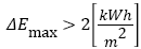and (Table 1) after a period of days a catastrophic earthquake can be expected

Obviously, it is not possible to use only one or two indicators similar to those described in this article for predicting earthquakes.

The problem of earthquake forecasting requires the set up and functioning of an online information system [7,14-16]. The system could be based on essential technologies: satellite systems [5], sensor systems, OLR trackers, fading of the wireless signals, electromagnetic emissions, land-based electricity undercurrents, tidal waves and other geophysical parameters in the active seismic geographical areas. The information system should include powerful computer configurations for signal processing. This system should be used for communication immediately before big earthquakes.

The authors express their acknowledgement for the financial support of this study by the grant COST Action ES1301 FLOWS.

References

- Venkatanathan N (2013) Outgoing long wave radiation anomalies associated with earthquakes of neighbouring region of India—A case study on earthquakes (Mw– 6.0) during the period of January 2012–November 2012. Int J Earth Sci Eng 6: 1750–1756.
- Venkatanathan N, Philipoff PH, Sreedharam V, Venkatachalapathy V (2016) Observation of pre-earthquake thermal signatures using geostacionary satellites. Journal of Applied Remote Sensing 10: 046004 .
- Venkatanathan N, Philipoff PH, Madhumitha S (2015) Outgoing longwave radiation anomaly prior to the big earthquakes: A study on the September 2015 Chile Earthquake. New Concepts in Global Tectonics Journal 3: 3.
- Jivkov V, Philipoff PH, Ivanov AN, Munoz M, Raikova G, et al. (2013) Spectral properties of quadruple symmetric real functions, Applied Mathematics and Computation, Elsevier 343-350 .
- Serebryakova ON (1992) Electromagnetic ELF radiation from earthquake regions as observed from low-altitude satellites. Geophys Res Lett 19: 91–94 .
- Freund FT (2003) Rocks that crackle and sparkle and glow: Strange pre-earthquake phenomena, J Scientific Exploration 17: 37-71 .
- Freund FT, TakeuchiA, Lau BWS, Post R, Keefner J, et al. (2004) Stress-induced changes in the electrical conductivity of igneous rocks and the generation of ground currents, Terr. Atm. Ocean Sciences (TAO)437-467 .
- Melbourne TI, Webb FH (2002) Precursory transient slip during the 2001 Mw = 8.4 Peru earthquake sequence from continuous GPS. Geophys Res Lett 29: 21 .
- Gousheva M, Danov D, Hristov P, Matova M (2009) Ionospheric quasi-static electric field anomalies during seismic activity in August–September 1981. Natural Hazards and Earth System Science 9: 3-15 .
- Pulinets S (2004) Ionospheric precursors of earthquakes: Recent advances in theory and practical applications. TAO, 2004. 15: 413-435.
- Pulinets SA, Boyarchuk K (2004) Ionospheric precursors of earthquakes. Springer, Berlin .
- Nenovski P, Chamati M, Villante U, De Lauretis M, Francia P (2013) Scaling Characteristics of SEGMA Magnetic Field Data around the Mw 6.3 Aquila Earthquake. Acta Geophysica 61: 311-337.
- Ouzounov D, Pulinets S, Hattori K, Kafatos M, Taylor P (2011) Atmospheric signals associated with major earthquakes. A multi-sensor approach, in frontier of earthquake short-term prediction study. Hayakawa M(ed) Nihon-Senmontosho-Shuppan, Japan510-531 .
- Cicerone RD (2009) A systematic compilation of earthquake precursors. Tectonophysics 476: 371–396 .
- Ouzounov D, Pulinets S, Romanov A, Tsybulya K, Davidenko D, et al. (2011) Atmosphere-ionosphere response to the M9 Tohoku earthquake revealed by multi-instrument space-borne and ground observations: Preliminary results. Earthquake Science 24: 557-564 .
- Pulinets S, Davidenko D (2014) Ionospheric precursors of earthquakes and global electric circuit. Adv Space Res 53: 709-723 .
Citation: Jivkov V, Natarajan V, Paneva A, Philipoff P (2017) Forecasting of Strong Earthquakes M>6 According to Energy Approach. J Earth Sci Clim Change 8: 433. DOI: 10.4172/2157-7617.1000433
Copyright: ©2017 Jivkov V, et al. This is an open-access article distributed under the terms of the Creative Commons Attribution License, which permits unrestricteduse, distribution, and reproduction in any medium, provided the original author and source are credited.
Select your language of interest to view the total content in your interested language
Share This Article
Recommended Journals
Open Access Journals
Article Tools
Article Usage
- Total views: 5601
- [From(publication date): 0-2017 - Dec 09, 2025]
- Breakdown by view type
- HTML page views: 4657
- PDF downloads: 944