Research Article Open Access
Identification of Hydrodynamics Coefficient of Underwater Vehicle Using Free Decay Pendulum Method
Yi DSL and Al-Qrimli HF*Faculty of Mechanical Engineering, Curtin University, 98009 Miri, Sarawak, Malaysia
- *Corresponding Author:
- Al-Qrimli HF
Faculty of Mechanical Engineering
Curtin University, 98009 Miri
Sarawak, Malaysia
Tel: +6085443939
Fax: +6085443837
E-mail: halqrimli@yahoo.com
Received Date: February 17, 2017; Accepted Date: March 22, 2017; Published Date: March 28, 2017
Citation: Yi DSL, Al-Qrimli HF (2017) Identification of Hydrodynamics Coefficient of Underwater Vehicle Using Free Decay Pendulum Method. J Powder Metall Min 6: 161. doi:10.4172/2168-9806.1000161
Copyright: © 2017 Yi DSL, et al. This is an open-access article distributed under the terms of the Creative Commons Attribution License, which permits unrestricted use, distribution, and reproduction in any medium, provided the original author and source are credited.
Visit for more related articles at Journal of Powder Metallurgy & Mining
Abstract
In this research paper, free decay method is proposed to identify the hydrodynamics coefficient of ROVs. This method is preferable for smaller-scale testing as it is a smaller and simpler method. In order to carry the experiment, an experimental rig is designed and constructed. The experimental rig is used to create an underwater environment which is important in the identification of the hydrodynamics coefficient. First, the equations of motion are formulated that can be used to describe the motion of pendulum given a set of parameters which included measured parameters such as mass and length of pendulum and also the unknown hydrodynamic coefficient which are added mass and the damping coefficients. Then, experiments are conducted where the displacement of the pendulum is recorded over time by using camera. The desired parameters are found by finding the combination of parameters such that the mathematical model fits the experimental data. Through this research project, it was found that the results obtained from this method are not reliable as claimed by a few authors. Although the data processing procedure was a success, the results obtained vary widely with different initial condition. This research project shows that in the current state, this method is not a good method in evaluating the hydrodynamic coefficient of the ROVs. Thus, an alternative method should be proposed or improvements should be made to produce a better result.
Keywords
Computational dynamics; ROVs; CAD design
Introduction
In the present study, Remotely Operated Vehicles (ROVs) are underwater unmanned robots that have been widely used in the ocean activities. ROVs are able to carry out tasks such as navigation, control and guidance for the deep ocean exploration which are beyond the capability of human beings. Thus, the identification of hydrodynamics coefficient of ROVs becomes a great concern [1]. Haidar F AL-Qrimli used many methods to identify the hydrodynamic parameters of ROVs. One of the most common method is Planar Motion Mechanism (PMM)/tow tank test. This method was introduced by authors [2-4] as a routine dynamics testing. PMM is capable of measuring the forces and moments in 6DOF which allows a complete identification. However, it is highly time-consuming and expensive to perform the test. According to Morrision and Yoerger [5], system identification method is also recommended to be used in the study of underwater vehicles. System identification method is the method of using onboard sensors and thrusters in the process of identification. Although there are many methods that can be used to identify the coefficient, free decay pendulum method is proposed to identify the hydrodynamics coefficient of ROVs because it is claimed by authors [2,3,6] that it is a repeatable and reliable method. As presented by Tan et al. [7], drag coefficient of any given models can be estimated by using fourth order regression method. By using CFD modelling, the model was subjected to pre-conditioning phase. The simulation was then run to obtain the drag profile in real-time. In their studies, it stated that the accuracy of the model is based on the frequency of trial runs and also the efficiency of the model’s sensors. It also stated that basic model of a cylinder was used to exhibit the accuracy and robustness of the proposed model. Thus, there is no proper experimental data to prove the validation of the data obtained. Further investigation such as identifying other fitting methods was also needed as stated in this paper to enable an accurate prediction. The aim of this project is to determine the hydrodynamic coefficient of ROV model through the free decay pendulum method.
Equation of Motion
The equations of motion are formulated from Newton’s second law. As the equation of motion can be expressed as: ƩF=ma, as it can be seen in Figure 1a.

Figure 1a: Free body diagram of pendulum under hydrodynamics forces.
Where ƩF is the total sum of forces on the body, ‘m’ is the mass and ‘a’ is the acceleration. In the pendulum experiment the considered forces include: hydrodynamic drag, buoyancy and weight. In this section the individual forces are discussed in detail leading to the formulation of the final equation of motion.
From the free body diagram,
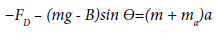 (1)
(1)
The equation of drag force:
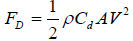 (2)
(2)
Since, s=Lθ
 (3)
(3)
Substituting equation (2) and (3) into (1), the total equation of motion:
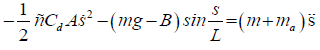 (4)
(4)
Free Decay Pendulum Experiment
The free decay pendulum experiment is a method of determining the hydrodynamic parameters of a submerged body. First the equations of motion are formulated that can describe the motion of the pendulum given a set of parameters which include measured parameters such as mass or pendulum length and also the unknown hydrodynamic coefficients which are added mass and the damping coefficients. Experiments are conducted where the displacement of the pendulum is recorded over time. The desired coefficients are found by finding the combination of parameters such that the mathematical model fits the experimental data.
Experimental rig
Experimental rig is one of the most important phases in this project. As the rig wasn’t an available facility to have due to the cost, a test tank was required to conduct the experiments. The tank is designed to be portable to allow us to move the tank easily from place to place. The external tank structure is made of joinable steel tubules with a PVC coated polyester fabric to contain the water. It is therefore disassemblable. The pendulum is mounted on a beam that spans the distance as it can be seen in Figure 1b.

Figure 1b: Experimental rig set up and the pendulum of the rig.
Experimental procedure
During the experiment, the pendulum is lifted to the starting position. The camera is started to begin the recording and at the same time the pendulum is released to decay in the water. After a short amount of time, the camera is stopped as the pendulum comes to at rest. The video recorded is processed by using image processing method to obtain the data and least squares fitting is applied to obtain hydrodynamic coefficients. The ROV can be seen inside the rig when its fill of water in Figure 2 using a GoPro camera to record the experiment. The images of the motion of pendulum are required for analyzing the hydrodynamics coefficient (Figure 2).

Figure 2: The ROV underwater in the rig.
Data Analysis
The experiment is carried out and a camera is used to record the video. Images of the video are obtained by splitting the video in frames. After that, the images are processed by using MATLAB program. In this experiment, the motion of the pendulum is represented by the coordinates of a dot. In order to find the coordinate of dots, circle detection is required. By using MATLAB software, image processing method is used to process the image of motion. First, the image is read by using loop function to repeat the image reading process. Next, the contrast of the image is changed to enable the program to identify the circles easier. The image is then cropped to minimize the error during image processing. The circle is detected by using function in MATLAB. Angle is determined by using MATLAB Atan2 function. The angle obtained is then converted into displacement by using Equation 3. Lastly, regression method is applied to compare the theoretical and experimental data. Least squares regression is a technique to match analytical models with experimental data. In order to do this, the algorithm estimates the combination of parameters that reduce the error between the data set and the model in the least squares sense. In this experiment, this method is used to compute the estimated added mass and drag coefficients.
Results and Discussion
From the total equation of motion there are few parameters which can be calculated or measured without carrying out the experiment. These known parameters are simplified in Table 1. This volume corresponds to a buoyancy force of 24.43N. Buoyancy acts in the opposite direction of the weight so their effects may be combined to simplify analysis. The experiment is carried out multiple times with varying initial displacements in both directions to have a better analysis of the experiment. All the data obtained are analyzed and shown in this section (Table 1).
| Parameters | Values |
|---|---|
| Mass(m) | 3.53 kg |
| Volume (V) | 0.0025 m3 |
| Density of water (ρ) | 1000 kg/m3 |
| Gravitational force (g) | 9.81 m/s2 |
| Length of pendulum (L) | 0.76 m |
| Frontal Area (A) | 0.0322 m2 |
| Buoyancy (B) | 24.43 N |
| Weight (mg) | 34.63 |
Table 1: Summary of known parameters and its values.
In order to ease the experiment, few assumptions were made such that the model is rigid and full submerged once in water. Water is assumed to be an ideal fluid that is incompressible, in viscid and irrational. The rod is assumed to be a point mass and frictional forces of the rod and pivot are negligible. The experiment results data is carried out multiple times with varying initial displacements in both directions to have a better analysis of the experiment. All the data obtained are analyzed and shown in this section. The result obtained by using initial position of 75°, the video of the motion is analyzed using Matlab software is shown in Figure 3. By using initial position of 20°, the video of the motion is analyzed using Matlab software. The result obtained is shown in Figure 4. In addition Figures 5-7 shows the initial positions of -15°, 5° and position of approximately -5° respectively. From observing the graphs obtained, it can be concluded that the data with larger initial position do not fit well with the model. This can also be proven by the values of RMS error calculated which also show that the data with larger initial position have higher value of error. However, the RMS error values, shown in Table 2, for all the data are relatively small which only range from 0.005 to 0.001. This shows that the data extracted from the free decay pendulum method can actually fit well with the model derived (Table 2 and Figures 3-7).

Figure 3: Graph showing data fitting of data with model of best fit for 75°.

Figure 4: Graph showing data fitting of data with model of best fit for 20°.

Figure 5: Graph showing data fitting of data with model of best fit for -15°.

Figure 6: Graph showing data fitting of data with model of best fit for 5°.

Figure 7: Graph showing data fitting of data with model of best fit for -5°.
| Initial position (°) | RMS error |
|---|---|
| 75 | 0.00376 |
| 20 | 0.00462 |
| -15 | 0.00321 |
| 5 | 0.00139 |
| -5 | 0.00111 |
Table 2: RMS error values.
From Table 3, the added mass obtained for initial position 75, 20, -15, 5 and -5 are 4.2577 × 10⁻¹⁴ kg, 19.266 kg, 3.0988 kg, 15.098 kg and 19.169 kg respectively while the drag coefficient calculated are 0.457, 2.999, 6.897 × 10⁻¹³, 6.903 × 10⁻¹³ and 6.896 × 10⁻¹³ respectively. By comparing these values, we can observe that the estimated values are not consistent and vary widely depending on the starting angle. The tests run at 5 and -5 degrees show the most consistency, this indicates that the output is highly sensitive to initial conditions (Table 3).
| Initial position (°) | Ma (kg) | CdA | Cd |
|---|---|---|---|
| 75 | 4.2577 × 10⁻¹⁴ | 1.4719 × 10⁻² | 0.457 |
| 20 | 19.266 | 9.6585 × 10⁻² | 2.999 |
| -15 | 3.0988 | 2.2208 × 10⁻¹⁴ | 6.897 × 10⁻¹³ |
| 5 | 15.098 | 2.2228 × 10⁻¹⁴ | 6.903 x10⁻¹³ |
| -5 | 19.169 | 2.2204 × 10⁻¹⁴ | 6.896 x 10⁻¹³ |
Table 3: Summary of experimental data.
Conclusion
This research project uses a free decay test to identify the added mass and the drag coefficient of the openROV robot. The data processing procedure was a success as it was able to extract displacement-time data from a video recording. Through the analysis of the experimental data, curve fitting routine was proven successful as it was able to match the data with the model well. This is proven by visual inspection of the graphs and also the low RMS values obtained. However, the results obtained shows that the parameter output is highly sensitive to initial conditions as a result, the estimated parameters vary widely. Thus, from this research project, it shows that the free decay method is not a good method in finding the hydrodynamic coefficient and added mass. The recommendation would be by improving the analytical model of the system which may include acceleration effects such as Basset force, time varying effects such as flow development and also others such as friction in bearings and pendulum arm.
Acknowledgement
I would like to express the deepest appreciation to Dr. Haidar Al-Qrimli and Mr. Zachary MacChesney for guiding and helping me throughout this research project. Besides, I would like to thank to the lab assistant for allowing me to conduct my experiment in the lab.
References
- Caccia M, Indiveri G, Veruggio G (2000) Modeling and identification ofopen-frame variable configuration unmanned underwater vehicles.IEEE Journal of Oceanic Engineering25: 227-240.
- Chin C, Lau M (2012) Modelling and Testing of Hydrodynamic Damping Model for a Complex-shaped Remotely-operated Vehicle for Control. J Marine SciAppl11: 150-163.
- Eng YH, Lau WS, Low E, Seet GGL, ChinCS (2008) Estimation of theHydrodynamics Coefficients of an ROV using Free Decay Pendulum Motion. Engineering Letters 16:3, EL_16_3_09.
- Goodman A (1960) Experimental techniques and methods of analysis used insubmerged body research. Third Symposium on Naval Hydrodynamics, Office of Naval Research.
- Morrision AT, Yoerger DR (1993) Determination of the Hydrodynamic Parameters of an Underwater Vehicle During Small Scale. Nonuniform, 1-Dimensional Translation. II 277-282.
- AL-Qrimli HF, Khalid KS, Abdelrhman AM, Mohammed ARK &Hadi HM(2016) A Review on a Straight Bevel Gear Made from Composite.Journal of Materials Science Research 5: 3.
- Tan KM, Lu T,Anvar A (2013) Drag Coefficient Estimation Model to Simulate Dynamic Control of Autonomous Underwater Vehicle (AUV) Motion. Paper presented in 20th International Congress on Modelling and Simulation Held in Adelaide, Australia, 1-6 December 2013. pp: 963-969.
Relevant Topics
- Additive Manufacturing
- Coal Mining
- Colloid Chemistry
- Composite Materials Fabrication
- Compressive Strength
- Extractive Metallurgy
- Fracture Toughness
- Geological Materials
- Hydrometallurgy
- Industrial Engineering
- Materials Chemistry
- Materials Processing and Manufacturing
- Metal Casting Technology
- Metallic Materials
- Metallurgical Engineering
- Metallurgy
- Mineral Processing
- Nanomaterial
- Resource Extraction
- Rock Mechanics
- Surface Mining
Recommended Journals
Article Tools
Article Usage
- Total views: 4128
- [From(publication date):
April-2017 - Aug 17, 2025] - Breakdown by view type
- HTML page views : 3068
- PDF downloads : 1060