Impact of Land-Sea Breeze and Rainfall on CO2 Variations at a Coastal Station
Received: 17-Apr-2014 / Accepted Date: 16-Mar-2014 / Published Date: 20-Jun-2014 DOI: 10.4172/2157-7617.1000201
Abstract
Carbon dioxide (CO2) observations collected at 5 min interval at Sriharikota during October 2011-January 2012 from the Vaisala GMP-343 sensor were averaged on an hourly basis. The baseline of atmospheric CO2 during study period is 382 ppm. Minimum (maximum) mixing ratios was observed during the afternoon (night times) indicating the role of photosynthetic activity and the atmospheric boundary on this parameter. Sriharikota being a coastal station, the land and sea breezes mainly control CO2 mixing ratios. The correlation between CO2 and the wind speed is significantly less during sea breeze than during land breeze in October, compared to other months, where the correlations are more during sea breeze. The less correlation during sea breeze in October is due to the heavy rainfall in this month during daytime.
Keywords: Carbon dioxide (CO2) mixing ratios; Rainfall impact; Land and sea breezes
7967Introduction
Carbon dioxide (CO2), one of the major Greenhouse Gases (GHG) in the atmosphere, plays a prominent role in climate change. The global mean concentration of CO2 in 2005 was 379 ppm, leading to a Radiative Forcing (RF) of +1.66 [± 0. 17] W m-2 [1]. Recently, the CO2 levels have gone up to a daily mean of 400 ppm in May 2013 at Mauna Loa, Hawaii [2]. Local meteorological and environmental factors control the CO2 mixing ratios. During night times, temperature inversions prevent thorough mixing of the atmosphere. There is also an absence of photosynthetic activity consuming CO2. Due to these two processes, CO2 mixing ratios increase at night. During the daytime due to increase in photosynthesis activity, CO2 mixing ratio decreases [3].
To understand the carbon cycle in the atmosphere, several surface CO2 measuring network stations have been established across the county under National Carbon Project (NCP). NCP is a component of Geosphere Biosphere Programme (IGBP) of the Indian Space Research Organization (ISRO). Under this program terrestrial, ocean and atmospheric components of carbon balance are studied. Instruments are installed to measure the atmospheric CO2 [3], flux measurements in forests [4] and in soil [5]. As a part of this program, GMP-343 is installed in 2011 at Sriharikota High Altitude Range (SHAR). Since this is a coastal station, we report the impact of the wind vector, particularly the land and sea breezes, on CO2 variations from October 2011 to January 2012. While pure water has pH of 7.0, normal rain is slightly acidic with pH range from 5.0-5.6 [6] because of dissolving of CO2 in water droplets forming a weak carbonic acid. The dissolution of CO2 in rain drop depends upon the partial pressure of CO2 and the atmospheric temperature. Since the study region influenced by North East (NE) monsoon, we also studied the impact of rainfall on CO2 mixing ratios.
Study Area And Instrumentation
The study region (Figure 1) in Sriharikota is a coastal Island, 0.5 km away from the coast of Bay of Bengal (BoB) and connects to an urban area with a road. This site has a large area of vegetation and trees with less pollution. The GMP-343 was installed at a height of 30 m from the ground on the top of a building. The sensor is mounted above the rooftop to insulate from the heating effects. It measures the atmospheric CO2 mixing ratio by utilizing the silicon based Non-Dispersive Infrared (NDIR) sensor to detect the absorbance of IR radiation by CO2. The instrument is calibrated at the factory with 5 known concentration of CO2 values (0-1000 ppm). The graph between the CO2 measured by the instrument and the standard values are shown in Figure 2. Most of our observations are below 500 ppm and the difference between two observations varies from 1 and 3 ppm. This calibration is carried out at 26.2°C and the pressure varying between 1016.4 to 1016.7 hpa. These differences are much within the permissible limit. As per the Vaisala standard calibration procedure, the accuracy of the instrument is ± 2 ppm for a temperature range of -40 to 60°C and for concentration range 0-1000 ppm. The precision of the instrument at 370 ppm with 30sec output averaging is ±1 ppm. The instrument (reference cylinder) drift in one year is ≤ 2% (± 0.5%) of the reading (Vaisala GMP-343 user guide and calibration report). The station has two towers of 100 m and 50 m. The 100 m tower has wind sensors at 100 m, 80 m, 60 m, 40 m, 30 m, 20 m and 10 m height. The 50 m tower has temperature and humidity sensors at 50 m, 32 m, 16 m, 8 m and 4 m. The continuous CO2 observations were collected through a panoptic data logger at 5 min interval. The technical details and schematic diagram of the instrument are given in [3]. These CO2 mixing ratios and wind vectors are analyzed for four months during October 2011 to January 2012.
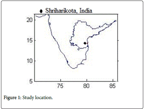
Figure 1: Study location.
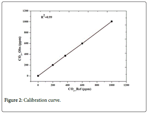
Figure 2: Calibration curve.
Methodology
The measurements were made using Vaisala made GMP-343 sensor. These values were recorded at 5min interval at 30 m height. The GMP-343 was well calibrated with standard CO2 gas cylinders and instrument bias was removed from the observations. CO2 observations were corrected for atmospheric moisture from Wagner [7] equation using saturated vapour pressure of CO2:
ln( p/pc) = (α1τ+α2τ1.5+α3τ3+α4τ3.5+α5τ4+α6τ7.5) Tc /T (1)
Where, p = es (saturated vapour pressure), Tc (critical temperature) = 647.096K, pc (critical pressure) = 220 64 kPa, a1 = -7.859 51783, a2 = 1.844 082 59, a3 = -11.786 6497, a4 = 22.680 7411, a5 = -15.961 8719, a6 = 1.801 225 02 and τ = 1-(T+273.15)/Tc
Relative Humidity (RH) = (e/es)*100 (2)
CO2dry=CO2wet/(1-0.001*e) (3)
The correction to be applied to the instrument measurements varies from 1.2 ppm to 14 ppm during October to January. The correction in October is more because of the more atmospheric water vapour in this month. Savitazky-Golay filter technique [8] was used to reduce the time series signal noise. This technique can be applied to any continuous and more or less smooth data with a fixed and uniform interval along the axis [9]. The 5 min observations have been averaged to hourly daily values. Along with the 100 m and 50 m tower observations, we have also computed 5-day back trajectory analysis at an altitude of 100 m for the study period using Hybrid Single Particle Lagrangian Integrated Trajectory (HYSPLIT) model [10].
Results And Discussions
Setting up the atmospheric CO2 background
To have a quality control of the data, setting the background level (baseline) is required. For this purpose, we first filtered all the data following Savitazky-Golay technique [8]. The original data (black curve) and the data after filtering (red curve) are shown in Figure 3. These filtered values are used to compute the hourly means. These hourly observations were checked for consistency and only those observations, where the difference between the two consecutive values is less than 0.5 ppm are considered (4 % of the observations were removed in this way). Then the regional background level (baseline) was computed as a means of the hourly data following Zhou [11]. Thus, the baseline of this region is 382 ppm with a standard deviation of 8.1 ppm.
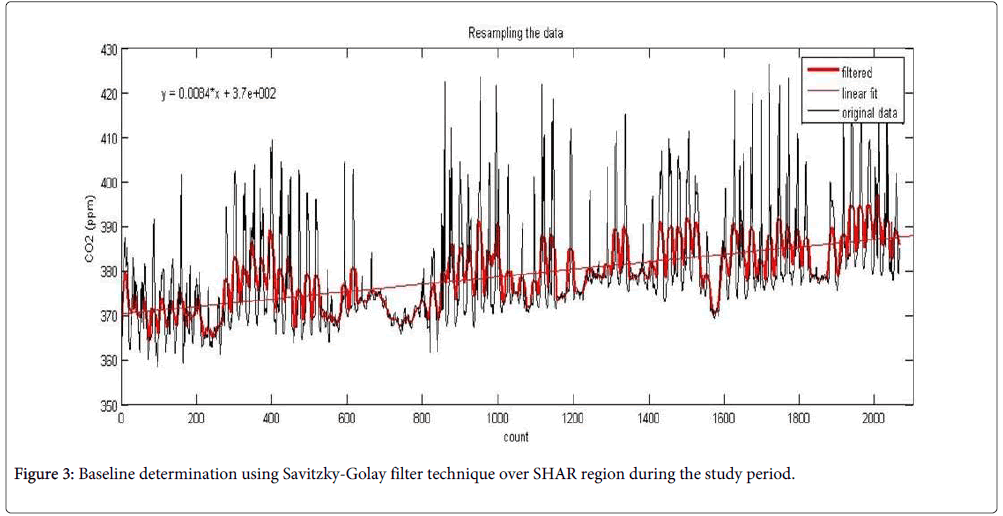
Figure 3: Baseline determination using Savitzky-Golay filter technique over SHAR region during the study period.
Diurnal variation of CO2
Diurnal variation of CO2 mixing ratios are shown in Figure 4. The diurnal variations are similar during all the months but with varying concentrations. The first peak (crest) in every plot is at around 0700 to 0800 IST, which is due to the accumulation of CO2 mixing ratios during early morning, before the sunrise. As the day advances the level of CO2 decrease gradually and reaches a minimum by afternoon (1300 IST to 1500 IST) due to high atmospheric mixing [12] and due to the increased photosynthesis activity. The mixing ratios again increase after the evening, after the sunset, peaking around 1900 IST-2100 IST due to the absence of photosynthesis activity besides wind effects, which will be discussed later. The maximum diurnal variation is during January 2012 with maximum value of 407 ppm at 0700 IST and minimum value of 380 ppm at 1500 IST. Similar diurnal variations are observed by Neerja [3,13] at Dehradun and Gadanki, India. Though the pattern remains almost same, the mixing ratios vary from month to month with January (November) having highest (lowest) values. Since the atmosphere is relatively calm and stable with frequent inversions during winter season, the high values are present during January and December compared to other months. November CO2 mixing ratios are less than those in October by ~10 ppm through the day. This could be due to high rainfall in October with more moisture content which in turn increases the wet correction and increases the value of dry CO2.
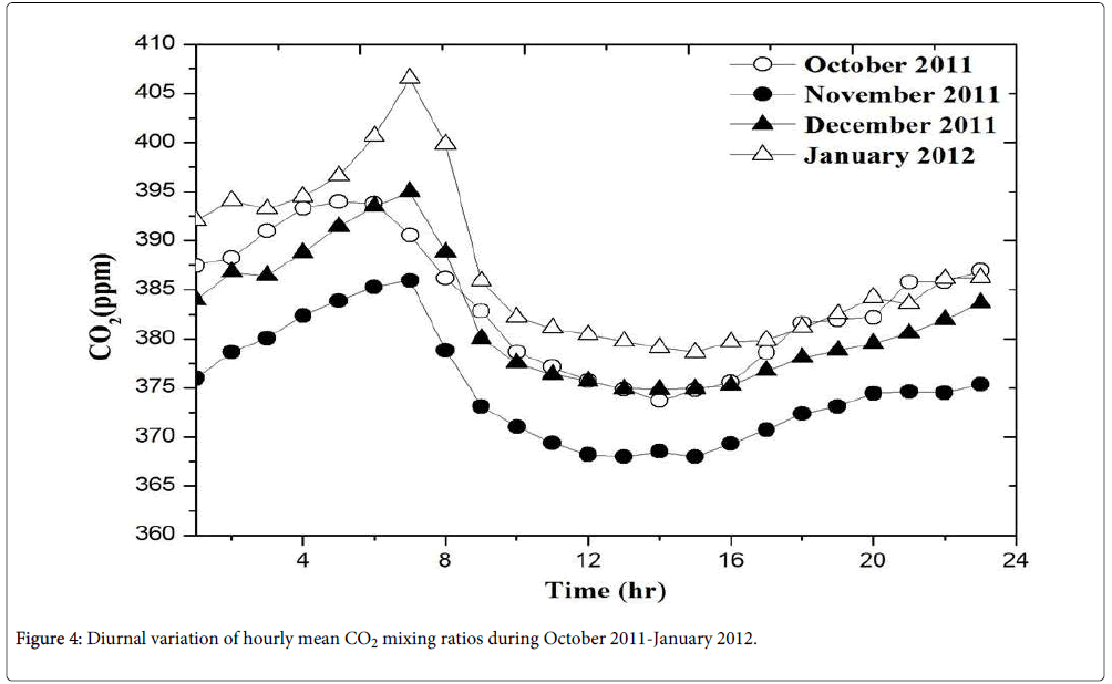
Figure 4: Diurnal variation of hourly mean CO2 mixing ratios during October 2011-January 2012.
Impact of wind vector on variation of CO2
Wind speed
The impact of wind speed on the CO2 mixing ratios varies from month to month (Figure 5). 76% (69%) of the variations in CO2 are due to wind speed in January (December) with less control of wind during October and November (44%). High winds have the scavenging effect besides reducing the stability of the atmosphere due to which high (low) concentrations are observed with low (high) winds. October and November being post monsoon months other factors like soil respiration and photosynthesis might have been controlling the CO2 mixing ratios due to which the percentage contribution of wind is less in these two months. The observations with maximum (minimum) mixing ratios of 407 ppm (361 ppm) have wind speeds of 1.68 m/s, (3.16 m/s). From this, we can conclude that the scavenging effect of wind magnitude plays a dominant role in controlling the CO2 mixing ratios at this coastal station.
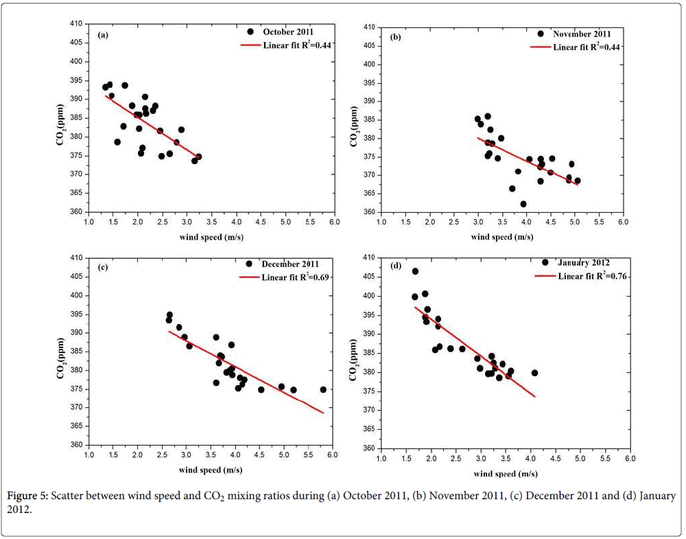
Figure 5: Scatter between wind speed and CO2 mixing ratios during (a) October 2011, (b) November 2011, (c) December 2011 and (d) January 2012.
Wind direction
Analysis of 100 m tower wind data shows that the prevailing wind direction during the study period at SHAR (Figure 6a) is from west-southwest [200°-340°] and east-northeast [20°-160°]. Besides analyzing the AWS winds, we have also computed the 5-day model vertical velocity air mass back trajectories at an altitude of 100 m (Figure 6b) for the study period using the HYSPLIT model for the same period. This analysis also reveals that the majority of winds are from northeast direction.
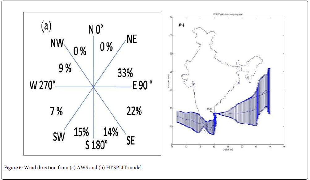
Figure 6: Wind direction from (a) AWS and (b) HYSPLIT model.
Impact of land and sea breezes
To study how land and sea breezes affects the CO2 mixing ratios, we considered all the winds coming from 00-1800 as sea breeze and those coming from 1800-3600 as land breeze and accordingly CO2 mixing ratios are divided. The demarcation of CO2 coming from land and sea is shown in Figure 7. Higher concentrations of CO2 are present during land breeze time. About 70% of the winds are from the Sea. Though coastal regions act as a source of CO2, the amount of CO2 concentrations from the ocean are less than those from land [14]. Thus, the sea breeze helps in reducing the CO2 concentrations at SHAR. Since sea breeze is stronger than land breeze, the scavenging effect of strong winds is another cause for these low concentrations during sea breeze time.
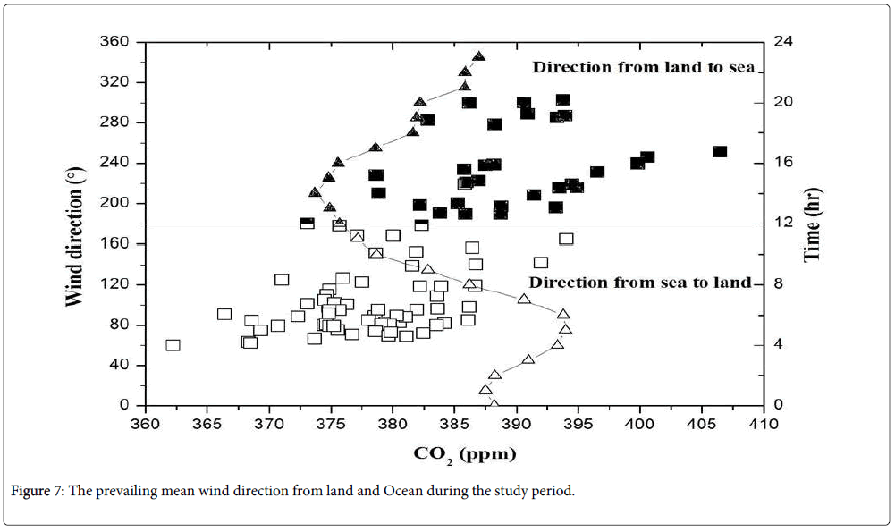
Figure 7: The prevailing mean wind direction from land and Ocean during the study period.
We carried out a dummy variable regression analysis considering months as the mutually exclusive variables. The coefficient of determination (R2) between the wind speed and the CO2 mixing ratio for all months together is 0.73, which otherwise is 0.52. This improvement shows the impact of seasonality on the mixing ratios. The monthly R2 and the y-intercepts with and without dummy variable analysis are given in Table 1. Monthly average wind speeds, mixing ratios and R2 between wind speed and CO2 mixing ratios during land and sea breezes separately for the four months is shown in Table 2. During sea breeze the mixing ratios (wind speeds) are slightly lower (higher) than those during land breeze. R2 during land breeze is less than that during sea breeze during November-January. The land breeze explains 58% to 82% variation in CO2 while the sea breeze explains 15% to 95%.
| Month | R2 | R2 | Y-intercept | Y-intercept |
|---|---|---|---|---|
| Without dummy analysis | With dummy analysis | Without dummy analysis | With dummy analysis | |
| Oct-11 | 0.42 | 0.65 | 409 | 402.2 |
| Nov-11 | 0.4 | 0.44 | 392 | 398.5 |
| Dec-11 | 0.64 | 0.68 | 398.2 | 408 |
| Jan-12 | 0.72 | 0.76 | 407 | 413.3 |
Table 1: Correlation between CO2 mixing ratios and wind speed with and without including months as a dummy variable.
| Month | Sea breeze | Land breeze | ||||
|---|---|---|---|---|---|---|
| Average Wind speed (m/s) | Average CO2 mixing ratio (ppm) | R2 | AverageWind speed (m/s) | Average CO2 mixing ratio (ppm) | R2 | |
| Oct-11 | 2.38 | 379 | 0.15 | 1.97 | 388 | 0.58 |
| Nov-11 | 4.22 | 371 | 0.66 | 3.59 | 377 | 0.45 |
| Dec-11 | 4.17 | 379 | 0.94 | 3.55 | 385 | 0.65 |
| Jan-12 | 3.01 | 385 | 0.95 | 2.37 | 390 | 0.82 |
Table 2: Correlation between CO2 mixing ratios and wind speed during land-sea breezes.
Impact of rainfall
To understand why R2 during October is significantly less during sea breeze contrary to the other three months, we analysed the hourly rainfall data since rainfall is another factor that scavenges the CO2. Depending upon the partial pressure of CO2 and the atmospheric temperature, CO2 dissolves in rain droplets producing a weak carbonic acid, H2CO3. Monthly total rainfall during the day (night) time during October 2011 to January 2012 is shown in Table 3. The comparatively heavy rainfall in October during daytime might have scavenged CO2 thus reducing its relationship with wind speed during sea breeze. Hence, wind speed could explain only 16% of the variations in CO2 during sea breeze in October.
| Month | rainfall (mm) | |
|---|---|---|
| Day | Night | |
| Oct-11 | 181.5 | 89.7 |
| Nov-11 | 6.52 | 7.9 |
| Dec-11 | 1.6 | 1.3 |
| Jan-12 | 0.74 | 0.02 |
Table 3: Rainfall during October 2011 to January 2012.
Summary And Conclusions
The continuous 5 min interval CO2 observations collected at SHAR, Sriharikota from Vaisala GMP-343 sensor were averaged on an hourly basis. The baseline of atmospheric CO2 during study period is 382 ppm. Minimum mixing ratios were present during the afternoon and maximum during nighttime reflecting the role played by the photosynthetic activity, the boundary layer dynamics and nighttime respiration. SHAR being a coastal station, the land and sea breezes mainly control CO2 mixing ratios. The mixing ratios have a seasonal behavior. Except during October 2011, the R2 between the wind speed and CO2 mixing ratios is more during sea breeze compared to that during land breeze for November, December and January. However, during October R2 between CO2 mixing ratios and wind speed is very less during sea breeze due to the very heavy rainfall in this month, which scavenged CO2 from the atmosphere.
Acknowledgement
This research work is carried as part of the Atmospheric CO2 retrieval and monitoring (ACRM) activity of the National Carbon Project (NCP). The authors thank their respective organizations for the support and encouragement during the progress of the work. The authors gratefully acknowledge NOAA Air Resources Laboratory (ARL) for the HYSPLIT trajectory model (http://ready.arl.noaa.gov/HYSPLIT_traj.php). The authors thank the anonymous referee for the constructive comments due to which the quality of the paper has improved.
References
- Monastersky R (2013) Global carbon dioxide levels near worrisome milestone. Nature 497:13-14.
- Sharma N, Nayak RK, Dadhwal VK, Kant Y, Ali MM (2013) Temporal Variations of Atmospheric CO2 in Dehradun, India during 2009. Air Soil Water Res 6: 37-45.
- Chanda A, Akhand A, Manna S, Dutta S, Hazra S, et al. (2013) Characterizing spatial and seasonal variability of carbon dioxide and water vapour fluxes above a tropical mixed mangrove forest canopy, India. J Earth Sys Sci 122: 503-513.
- Patel NR, Dadhwal VK, Saha SK (2011) Measurement and scaling of Carbon Dioxide (CO2) exchanges in wheat using flux-tower and remote sensing. J IndSoc Remote Sensing 39: 383-391.
- Wiley JD, Bennett RI, Williams JM, Denne RK, Kornegay CR, et al. (1988) Effect of storm type on rainwater composition in southeastern North Carolina. Environ SciTechnol 22: 41-46.
- Wagner W, Pruss A (1993) International Equations for the Saturation Properties of Ordinary Water Substance. Revised According to the International Temperature Scale of 1990. J PhysChem Ref Data 22: 783-787.
- Savitzky A, Golay MJ (1964) Smoothing and differentiation of data by simplified least squares procedures. Anal Chem 36: 1627-1639.
- Chen J, Jonsson P, Tamura M, Gu ZH, Matsushita B, et al. (2004) A simple method for reconstructing a high-quality ndvi time-series data set based on the Savitzky-Golay filter. Remote Sensing Environ 91: 332-344.
- Draxler RR, Rolph GD (2013) HYSPLIT (HYbrid Single-Particle Lagrangian Integrated Trajectory) Model. NOAA Air Resources Laboratory, College Park, MD, USA.
- Zhou L, Tang J, Wen Y, Li J, Yan P, et al. (2003) The impact of local winds and long-range transport on the continuous carbon dioxide record at Mount Waliguan, China. Tellus Series B ChemPhy Meteor 55: 145-158.
- Verma RL, Sahu LK, Kondo Y, Takegawa N, Han S, et al. (2010) Temporal variations of black carbon in Guangzhou, China, in summer 2006. AtmosChemPhy 10: 6471-6485.
- Sharma N, Dadhwal VK, Kant Y, Mahesh P, Mallikarjun K, et al. (2014) Atmospheric CO2 Variations in Two Contrasting Environmental Sites Over India. Air, Soil Water Res 7: 61-68.
- Sarma VS, Krishna MS, Rao VD, Viswanadham R, Kumar NA, et al. (2012) Sources and sinks of CO2 in the west coast of Bay of Bengal. Tellus Series B ChemPhy Meteor 64: 1-10.
Citation: Mahesh P, Sharma N, Dadhwal VK, Rao PVN, Apparao BV, et al. (2014) Impact of Land-Sea Breeze and Rainfall on CO2 Variations at a Coastal Station. J Earth Sci Clim Change 5: 201. DOI: 10.4172/2157-7617.1000201
Copyright: © 2014 Mahesh P, et al. This is an open-access article distributed under the terms of the Creative Commons Attribution License, which permits unrestricted use, distribution, and reproduction in any medium, provided the original author and source are credited.
Select your language of interest to view the total content in your interested language
Share This Article
Recommended Journals
Open Access Journals
Article Tools
Article Usage
- Total views: 19187
- [From(publication date): 8-2014 - Aug 19, 2025]
- Breakdown by view type
- HTML page views: 14339
- PDF downloads: 4848