Long-Memory and Fractal Trends in Variations of Environmental Radon in Soil: Results from Measurements in Lesvos Island in Greece
Received: 04-Apr-2018 / Accepted Date: 16-Apr-2018 / Published Date: 24-Apr-2018 DOI: 10.4172/2157-7617.1000460
Abstract
This paper presents evidence of trends of fractal properties and long memory in three-month variations of radon in soil, in Lesvos Island, Greece. The methodology employed consists of sliding-window (a) detrended fluctuation analysis, (b) fractal analysis, (c) rescaled range analysis and (d) fractal dimension analysis with the methods of Higuchi, Katz and Sevcik. During measurements two mild earthquakes occurred in the vicinity. The results of the detrended fluctuation analysis revealed four peaks with slopes between 1.2 and 1.5. The fractal analysis method resulted in three peaks with persistent power-law exponent values in the range 2.2 and 3.0. The rescaled-range analysis indicated persistent Hurst exponents between 0.7-0.9 and in some segments, between 0.9-1. The fractal dimension analysis showed four peaks with fractal dimensions in the range 1.3-2.0 (Higuchi and Katz methods) and 1.0-1.5 (Sevcik method). The results were compared in terms of conversion to Hurst exponents. Several persistent segments were addressed, along with persistency-anti-persistency switching instances. Potential geological sources are discussed and analyzed.
Keywords: Fractals; DFA; Spectral fractal analysis; Fractal dimension; Radon in soil; Earthquakes
Introduction
Earthquakes are disastrous phenomena with extremely negative impacts on society and economy. The earthquakes are detrimental not only because they inevitably occur when specific geological conditions are met, but also because their prediction is still hard and painstaking [1-3]. Earthquake forecasting is a challenging topic among the scientific community, with numerous reports on the pursuit of credible and indisputable precursors [2,3-5]. Despite the complexity in delineating the various stages of the generation of earthquakes, there are many papers presenting significant work on features hidden in preseismic timeseries which may signal the emergence of a forthcoming earthquake [6-41]. Generally, at some phase during the earthquake preparation process, some type of pre-earthquake activity is expected, which can hopefully be detected by recurrent observations made in the vicinity of the earthquake's epicenter, or near the area of the displacement or fracture [5]. Earthquake prognosis is multifaceted a-priori and, ideally, should provide estimates of occurrence time, epicenter and magnitude, especially for strong earthquakes [2,3,34]. The earthquake prognosis has been viewed under different aspects. One aspect is the discrimination in five prognosis categories [1,3,33-35]: (a) preparation where maps of all the possible focal areas with potential magnitude sizes and forecasting periods are generated; (b) long-term prognosis of forecasting period up to 10 years; (c) intermediate prognosis with forecasting period up to 1 year; short-term prognosis forecasting period from a week up to a month; (e) immediate prognosis, in which a point prediction is made, viz. within a day or less.
This categorization is guided by the up-to-date level of physical understanding of the geological mechanisms leading to earthquakes and by the needs of society for a scientifically based preparedness before the occurrence of a strong earthquake. Another aspect has been reported [1]: long-term prediction between 10 and 100 years; intermediate prediction between 1 and 10 years; short-term prediction. The short-term prediction is considered of the highest rank as far as safety of the general population is concerned, in particular, in very seismic areas. In either prediction scheme, there has not been established one-to-one correspondence between specific seismic events and recordings anomalies [17,26-36] and this should be emphasized. Radon-222 (henceforth, radon) has been employed since many years for the prognosis of earthquakes [2,34]. Radon is an inert gas which is produced by the radioactive decay of 238 U series with a half-life of 3.86 days [42].
As radon decays, it is dissolved in the soil’s pores and fluids, as well as, in surface and underground water and, most importantly, in the atmosphere [42]. Radon in water and soil can migrate to short or long distances at measurable levels [2,43]. Due to this property, several researchers have reported radon alterations in groundwater, soil gas, atmosphere and thermal spas, prior to earthquakes [2,26-28,31-33,44- 54]. These alterations have been identified as potential short-term earthquake precursors [2,34,35]. Despite the related research, it should be emphasized that there is no universal model to describe the various geo-physical phases prior to the occurrence of an earthquake [17,26-35]. Due to this, the scientific community still debates the precursory value of the numerous reports of radon anomalies detected prior to intense or mild earthquakes [17,26-35]. On the contrary, several publications have presented evidence for the formation of strict criteria to identify hidden pre-earthquake patterns in the pre-seismic time-series on the basis of the concepts of fractality, self-organization and block entropy via symbolic dynamics [1,2-42]. Especially regarding radon emissions, recent papers have revealed fractal and self-organized critical (SOC) characteristics hidden in radon anomalies prior to significant earthquakes in Greece [26-28,31-33]. Moreover, pre-earthquake fractal characteristics of a three year radon signal have been explored through the method of Multifractal Detrended Fluctuation Analysis (MFDFA) [54]. The new methodologies employed in the radon papers of the last decade [26-28,31-33] e.g. the wavelet spectral fractal analysis, the Rescaled Range (R/S) Analysis, the Detrended Fluctuation Analysis (DFA) and the entropy analysis, have revealed self-affine persistentantipersistent behavior of the investigated radon anomalies similar to the ones of the pre-seismic electromagnetic disturbances in the ULF, LF and HF ranges [31,35].
This paper focuses on a three- month signal of radon in soil (Figure 1) measured by a radon station installed at the campus hill of the University of the Aegean, Lesvos, Greece (UALG) (39.05 0N, 26.57 0E) (Figure 2). The recorded radon signal included specific radon concentration anomalies which were elevated compared to the background values. Both radon anomalies and background concentration values were comparable to the anomalies and the background values of a previous experiment [27] at the same site and under identical recording methodology. The radon signal of the UALG station [27] was derived prior to a mild earthquake of the near area (ML = 5.0, 38.92 0N/24.97 0E, 2008-03-19) and was analyzed through several different techniques that are well known to reveal the chaotic and Self Orginized Critical (SOC) features of time-series. The employed techniques in publication [27], were the spectral fractal analysis, the R/S analysis, the DFA and several entropic measures applied through the concept of symbolic dynamics. All these techniques indicated that the reported anomalies in publication [27] were, most probably, due to the nearby mild earthquake of 2008-03-19. In the case of the present signal (Figure 1), several similarities were identified as with the case of the signal of publication [27]: Radon anomalies were clustered in a focused time period of the signal; The recording period, was accompanied by a mild seismic activity including only two mild earthquakes (4.0< ML < 5.0 ) in the vicinity (Table 1 and Figure 2) and no other event of greater magnitude; (c) the background of the signals was comparable.
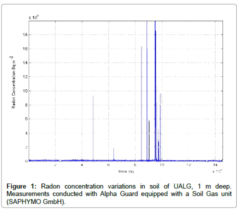
Figure 1: Radon concentration variations in soil of UALG, 1 m deep. Measurements conducted with Alpha Guard equipped with a Soil Gas unit (SAPHYMO GmbH).
| Event | Date (GMT) | Time (GMT) | Location | Latitude (°N) | Longitude (°E) | Magnitude (L) | Depth (km) |
|---|---|---|---|---|---|---|---|
| 1 | 10-09-2015 | 08:12:44 | 68,3 km N of Mitilini | 38.78 | 26.21 | 4.1 | 39 |
| 2 | 26-10-2015 | 19:50:05 | 33.4 km S of Mitilini | 38.87 | 26.19 | 4.6 | 46 |
Table 1: Seismic events during the analysis period (September 2-October 31/2015). Color-Schema identifier in Figure 1 according to the Institute of Geodynamics of the National Observatory of Athens.
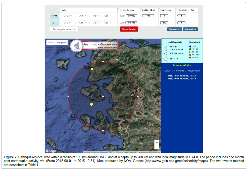
Figure 2: Earthquakes occurred within a radius of 100 km around UALG and at a depth up to 200 km and with local magnitude M L >4.0. The period includes one month post-earthquake activity, viz. (From 2015-08-01 to 2015-10-31). Map produced by NOA, Greece (http://www.gein.noa.gr/en/seismicity/maps). The two events marked are described in Table 1.
Taking into account the analysis methodology of the radon signal of publication [27] and of the other pre-earthquake radon time-series [26-28,31-33], this paper focuses on the delineation of hidden fractal, long-memory and SOC characteristics of the most recent radon signal recorded by UAGL (Figure 1). For direct comparison with publication [27], analysis is reported with the techniques of power-law spectral fractals, R/S, DFA and Hurst exponents. As a step further, analysis is reported on the time evolution of the fractal dimension calculated directly with the Higuchi, Katz and Sevcik methods. As supported in previous publications of the reporting team [6,7,26-36] and others [15- 17], this multifaceted approach is advantageous, because it provides different methodological aspects to reveal the chaotic, fractal and longtrends hidden in time- series. The consideration of viewing these trends as a potential pre-earthquake footprint is discussed and the possible geophysical explanations are presented.
Materials and Methods
Earthquake activity
The main period of the investigation lasted 119 days, viz, it started on June 2, 2015 and ended on September 30, 2015. A similar intermediate period of investigation was followed in all the previous papers of the team [26-28,31-33] for the analysis of the preseismic radon disturbances. To study the post seismic activity, 31 more days of earthquake activity were additionally included, namely the days from October 1, 2015 to October 31, 2015. During the whole period of investigation, only two earthquake events occurred in a circular area of radius 100 km around the UALG station (39.05°N, 26.57°E) (Figure 2). As shown in Table 1 the two events were mild since their local magnitudes M L were greater than 4.0 but lower than 5.0. Their distances from the UAGL station were 33 km and 68 km and this should be emphasized.
Instrumentation
Radon in the soil of UALG site was measured by Alpha Guard (AG) (SAPHYMO GmbH) [55] a high-precision instrument equipped with an appropriate unit designed for pumping and measurement of radon in soil gas (soil gas unit) [55,56]. The soil gas unit consists of a 1 m soil gas probe, an exterior steel tube with hammering head, an interior tube with adapter for tube connections, diverse sealing rings for the probe tip and filters which prevent the entry of moisture and progeny nuclei [26,56]. After driving the exterior steel tube at a depth of 1 m by hammering, the interior tube was plunged inside a cylindrical inner gap existing inside the exterior steel tube, placing in this way, the interior tube inlet at a depth of 1m. Previous experimentation showed that this installation minimizes the meteorological influences of the measurement of radon in soil [26,56]. The interior tube was connected through radon -tight tubes with radon progeny and moisture filters [26,56]. The whole set-up was connected to a radon tight pump (Alpha Pump, SAPHYMO) which was further connected with the AG through an input flow adapter and, continuously pumped soil gas into the AG [26,56]. The driven soil gas escaped the AG through an output flow adapter. To maximize radon flux and enhance, hence, the detection efficiency, pumping during measurements was performed at the maximum available rate of 1 L min 1 [26,56]. Radon concentration of soil was measured under a special measuring mode (flow mode). In parallel the atmospheric pressure (AP), relative humidity (RH) and temperature (T) were continuously monitored through special sensors. The whole setup was connected to a Pentium III PC operating under a Windows XP OS handling the AG through a Microsoft DOS software (AVIEW, Genitron Ltd.) licensed for the specific instrument of the study. The overall system constituted the radon station.
Results And Discussion
(Figure 3) presents the 60 db wavelet scalogram of the radon signal of Figure 1 in a segment between 8 × 10⁴ min and 11 × 104 min from the beginning of measurements, viz, between day 55 and 76, namely, between July 27 and August 17, 2015. The scalogram was generated by employing a logarithmic 256-scale Gabor filter. It is important to emphasize the following issues: The scalogram of the baseline of the signal samples did not exhibit high variability. This can be characteristically observed between sample 20,000 and 30,000 in (Figure 3). Importantly, this baseline scalogram exhibited a repeated scale texture constituting of a certain part of the decibel (db) range which is associated with the fGn class [27-35]; (b) The radon anomalies in the scalogram of Figure 3 lasted approximately from sample 2,500 to sample 11,000, i.e., about 6 days. The scalogram of the anomalies contained db information in the whole scale range, with the main power being allocated in the small scales, viz. the high spatial frequencies. Investigators [15-17] have declared this as a footprint of earthquake generation and significant for fractal fracturing systems [26-36]; (c) The background variations of radon in soil of the UALG site, exhibited characteristically different behavior in the wavelet domain than those of the anomalous parts. The scalograms of the background presented more power at the high frequencies and, most importantly, similar db profiles. This has been addressed at the same site previously [27] and in other preseismic signals of radon in soil [28-36]. (d) The scalogram of the environmental parameters (simultaneously recorded) was comparable to that of the radon background. This indicates that the findings of (b) above cannot be attributed to environmental parameters. Similar findings were also reported in previous publications [26,31,35].
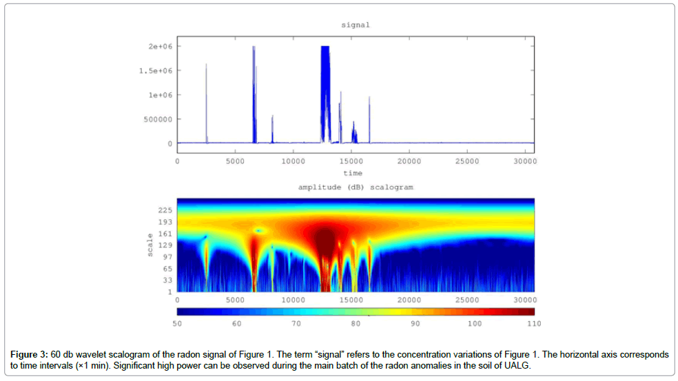
Figure 3: 60 db wavelet scalogram of the radon signal of Figure 1. The term “signal” refers to the concentration variations of Figure 1. The horizontal axis corresponds to time intervals (×1 min). Significant high power can be observed during the main batch of the radon anomalies in the soil of UALG.
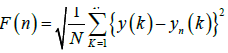
It is accepted that, while earthquakes are in the preparation stage, complex processes emerge, that are characterized by long-range powerlaw correlations and time-series with erratic fluctuations and scaleinvariant behavior [38]. Many times, there are inherent non-stationary patterns in the preseismic time-series associated with repeated temporal patterns [26-35,38], pseudo-sinusoidal trends [38], noise and sources of other origin. In such non-stationary signals, the traditional methods, e.g., auto-correlation and spectrum analysis cannot be used [57-60]. On the other hand, DFA has been proved to be a very powerful and robust technique suitable for identifying long-lasting power-law connections, not solely in non-stationary signals, but also, in noisy, randomized and short signals [15,31,38,61-69]. DFA has been utilized effectively in a variety of cases with scale-invariant behavior, as for example, in meteorology [70], climate temperature fluctuations [71], DNA [61], economics [72], circadian rhythms [67], heart dynamics [73], pre-earthquake activity of SES [37,38], electromagnetic disturbances of the MHz range [31,35] and preseismic variations of radon in soil [31,35]. In the above consensus and taking into account the previous work [28,31,35], DFA was applied to the radon timeseries of Figure 1. The corresponding results are presented in Figure 4. To derive this figure the steps described in previous papers [28,31,35] were followed. In brief: (I) The radon time-series (symbolized as yi, i = 1,....,N), was integrated according to (1).
 (1)
(1)
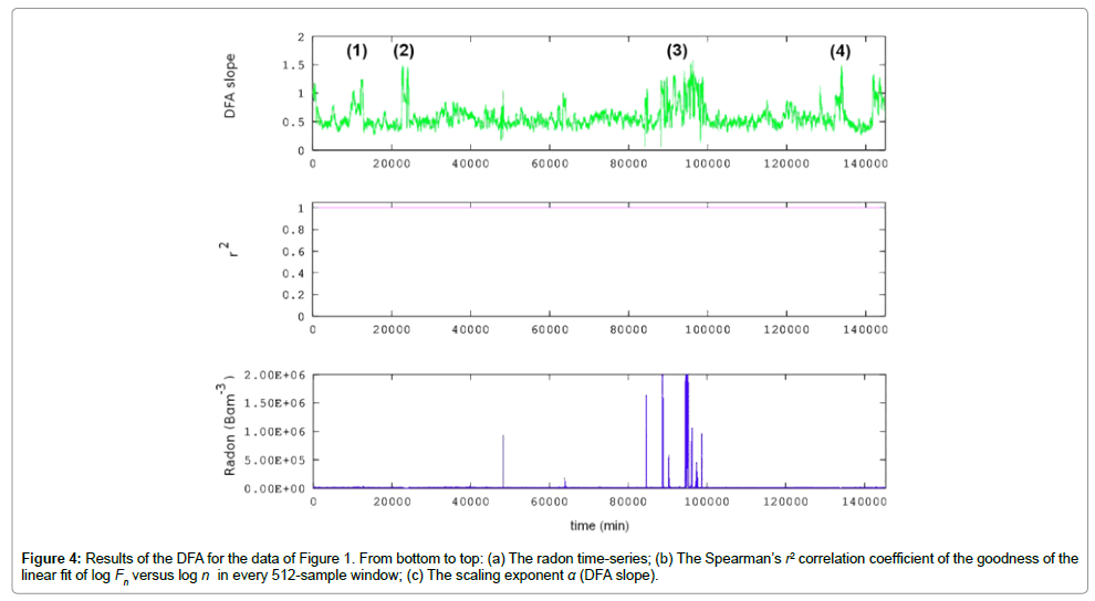
Figure 4: Results of the DFA for the data of Figure 1. From bottom to top: (a) The radon time-series; (b) The Spearman’s r2 correlation coefficient of the goodness of the linear fit of log Fn versus log n in every 512-sample window; (c) The scaling exponent a (DFA slope).
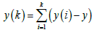
where k (integer) points to the different time scales n and y equals 12.8kBq .m-3 is the radon average value (background) of Figure 1 without any peaks. (II) The integrated signal of (1) was segmented into equal non-overlapping bins of length n, within which, a line was fitted representing the local trend (symbolized as yn (k)). The detrended signal ydn(K)was calculated in every bin n as:
 (2)
(2)
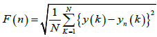
The root-mean-square rms fluctuations F n of the integrated and the detrended time-series was calculated as:
 (3)
(3)
Steps (I)-(III) were iterated for a wide range of bins, seeking a power-law relationship
 (4)
(4)
by fitting logF n versus log n to a line and calculating the scaling exponent a (slope) and the corresponding r 2 (Spearman's square) of the fit. (V) The procedure (I)-(IV) was computationally repeated in overlapping segmented portions of yi of size 512, shifted by 1 sample each (sliding-window technique) until the end of the signal (final window's last sample equal to N) [28,31,35].
The profile of the scaling exponent a in Figure 4 differs from the one of the radon time-series. This is characteristically shown in areas (1), (2) and (4), which exhibited a anomaly, but, without direct links to radon anomalies. As mentioned, these areas correspond to implicit non-stationary patterns in the preseismic radon time-series. Due to its robustness [38,69], DFA manages to identify such implicit patterns and, most importantly, to reveal also areas of hidden long-memory trends, as those of areas (2), (3) and (4). In these areas, the DFA slopes a of several segmented 512-sample windows, were greater than 1.4 (note that the a -value from the fit in a certain window, corresponds to a single value in the y-ordinate). As discussed in previous papers [16,29,31,35], these values can be considered as a trace of a forthcoming earthquake. Emphasis should be placed especially on area (3), since this exhibited (a) the longest duration, (b) high DFA slopes and, most importantly (c) direct link to radon anomalies. The outcome (c) has been observed also in pre-seismic time series of radon in soil of Ileia and UALG [16,29,31,35], while it is not usually valid for electromagnetic timeseries [16,17,26-35].
As discussed above and in several other related publications [11,12,19,23,25,31-35,37,38,40-42,44,47-49,55-59], while earthquakes are in the preparation phase, the associated physical systems exhibit scale-invariant behavior and long-range power-law correlations associated with complex connections between space and time and characteristic fractal structures. As these systems are driven toward the final catastrophe, they pass from states of self-organization and spatiotemporal fractal organization [57]. The scale-invariant, long-range power-law correlations of the Self-Organized Critical (SOC) states of the seismic fractal systems, may be revealed also through the powerlaw fractal analysis of the time-series [11,12,19,23,25,31-35,37,38,40-42,44,47-49,55-59].
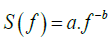
More specifically, if a time signal A ti is a temporal fractal, its power spectral density (PSD), S f, will obey a power-law of the form
 (5)
(5)
where a is the spectral amplification and f is frequency of a transform (the reader should note here that the spectral amplification a is different from the DFA scaling exponent a). The spectral amplification a quantifies the strength of the spectral components f following the power law and the spectral scaling exponent b is a measure of the strength of the time correlations. It is significant to recognize segments with distinct changes of the scaling exponent b since such changes are reported to emerge before major earthquakes [23,24,31-35,37,38,44,45,48,49,52,56-59].
Figure 5 presents results from the fractal analysis method. To derive the data, the methodology followed was [11,12,27,31,35,37-41,44-49]: (A) The radon time-series was divided in windows of 512 samples, as with the DFA data of Figure 4. According to the previous radon related research [27,31,35] this segmentation can reveal the fractality of radon signals; (B) In each segment the PSD of the signal was calculated with the Morlet base function to obtain the Sff combinations. In each segment a least square fit was applied to the log S f log f representation of (5). The frequency f was the central frequency of the Fourier transform of each Morlet scale. Successful representations were considered those that exhibited squares of the Spearman's correlation coefficient above 0.95. What makes Figure 5 important is that it displays long-memory trends that require further attention. Prior to commenting on that it is crucial to emphasize the following issues: If power-law b values are between 1 b < 1, the corresponding time-series follow the fractional Gaussian noise (f Gn) class; If b =1, the fluctuations of the processes do not grow and the related system is stationary; If 1< b3, the timeseries constitute a temporal fractal following the fractional Brownian motion (fBm) class; Values 1< b< 2 imply antipersistency; If b = 2, the system follows random dynamics of no memory (random-walk); (vi) Values 2< b< 3 suggest persistency with faster fluctuation accumulation than in fBm. Accounting for these facts, it can be supported that the preseismic radon-signal exhibited successful (r2>0.95) fractal epochs, however, scattered in time. Despite the scattered behavior, there are successful epochs with high power-law-b values above 1.7, namely well away randomness. These values are well associated with the fBm class [11,12,27,31,35,37-41,44-49] and have been proposed as noteworthy pre-earthquake signs. Importantly, segments can be observed with b -values above. These are associated with persistency and have been proposed by some researchers [8,9,11-17,21-25], as the most significant precursory sign of the inevitable phase of the earthquake occurrence. According to other researchers [11,12,26-35], the most important sign is the change between anti-persistency and persistency – which can be observed in all marked areas.
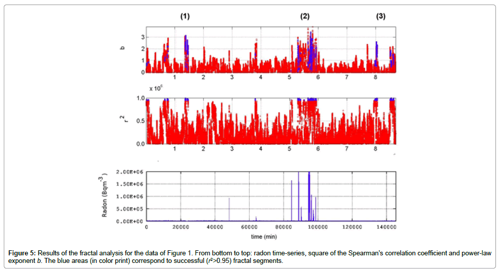
Figure 5: Results of the fractal analysis for the data of Figure 1. From bottom to top: radon time-series, square of the Spearman's correlation coefficient and power-law exponent b. The blue areas (in color print) correspond to successful (r2 >0.95) fractal segments.
Comparing the outcomes of Figures 4 and 5, it is very significant to emphasize those areas (2), (3) and (4) of Figure 4 coincide with areas (1), (2) and (3) in Figure 5. Importantly, the area (2) in Figure 5 is linked to the radon anomalies, as the area (3) of Figure 4. These simultaneous findings reinforce the view that these areas include pre-seismic signs of the earthquakes of Table 1. It should be noted though- as emphasized up this point- that it is very hard to find a one-to-one link between a certain sign and an event. Despite that only one event occurred during the main period of investigation, it is most probable that areas (2), (3) of Figure 4 and areas (1), and (2) of Figure 5, could be a premonitory sign of the preparation phase of the nearby earthquake number 1 of Table 1. Similarly, area (3) could be a pre-seismic sign of earthquake number 2 of Table 1.
Figure 6 presents the results of the R/S analysis of the radon-series of Figure 1. To generate this figure the procedure followed in previous publications [29,32,35] was followed. In brief: (A) The average of the radon time-series (here symbolized as X (n)n = x (1), x (2), x (n), where n (n = 1, 2,N) and for this case, N equals 512, the window size of the analysis) was calculated as:
 (6)
(6)
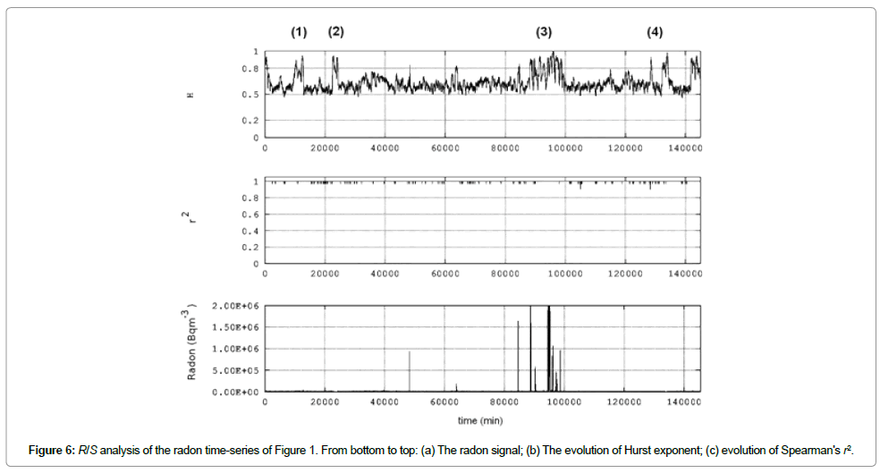
Figure 6: R/S analysis of the radon time-series of Figure 1. From bottom to top: (a) The radon signal; (b) The evolution of Hurst exponent; (c) evolution of Spearman's r2.
From (6) the accumulated departure of the radon time-series was calculated as [28,29,57-59]:
 (7)
(7)
From y (n, N), the range R(n) was calculated according to (8) [28,29,57-59].
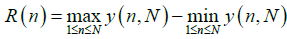 (8)
(8)
From X(n) and XN the standard deviation, S (n), was calculated as:
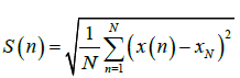 (9)
(9)
Taking into account that R/S ratio is expected to follow a power-law relation
 (10)
(10)
where H is the Hurst exponent and C is a constant of proportionality, a linear fit was applied to
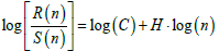 (11)
(11)
from which H (Hurst exponent) was calculated through the fit. The strength of the fit was checked, as with the DFA and fractal analysis, by calculating the square of the Spearman's correlation coefficient; (E) The window was shifted forward one sample (sliding window technique) and the above steps were repeated until the end of the radon signal. Prior to commenting in Figure 5, it is significant to discuss first some issues related to the H - exponent values which are calculated by (11). Hurst exponents are very important because their calculation reveals the existence or not of long-range dependencies in time-series [67,70], unfolds their smoothness and estimates if the related phenomenon is a temporal fractal [74]. Due to the significance, Hurst exponents have been utilized in many fields [57,58,71-80] including the study of pre-seismic precursors [15,26,32,35]. Regarding H, the following are valid:If 0.5< H< 1, the related time-series exhibit long-lasting positive autocorrelation. This implies that a high present value will be possibly followed by a high future value and this tendency will last for long timeperiods in the future (persistency) [26-36]; If 0< H< 0.5, the time-series exhibits long-term switching between high and low values. This means that a low present value will be followed by a high future value, while a high present value will be followed by a low future value. This lowhigh switching will continue into the future for many samples (antipersistency) [26-36]; If H = 0.5 the time-series profile is completely uncorrelated.
Accounting for the above facts, (Figure 6) reveals very important information about the radon time series of Figure 1. As can be observed, all H values were in the range 0.5-1. This means that the radon time-series had underlying memory associated with persistency. Most importantly, as with (Figure 4), four areas are identified with significantly increased H values above 0.8 in several segments. As with the previous interpretations, the areas (1- 3) could be precursory of the nearby earthquake number 1 of Table 1, while area (4) could be a sign of earthquake number 2. Most important is however that, within these four areas, the radon signal when increasing continued to increase and where it decreased, it continued decreasing (persistent behavior). Especially during Hurst exponent peaking, the radon concentrations referred to their past values so as to define their present values and, from these, their forthcoming values. This implies that the Hurst anomaly generating system was not at all random. It could be generated by cracks propagating within the earth's crust, in a manner, that crack batches of the past, were sources of present crack batches and these sources of upcoming crack batches. In another viewpoint, the cracks of the past were organized to generate the cracks of the present and then of the future, producing a self-organized backbone of asperities [14-17]. Researchers have pinpointed this as a signature of impeding earthquakes [14-17,21-35]. The crack propagation or the asperities backbone could be the inner earth's causes of radon anomalies through its exhalation or inhalation due to the sign of the pressure differential. This is characteristically seen in area (3) in which the radon anomalies coincide with those of the Hurst exponent. It is very important to note here that similar behavior has been addressed in anomalous concentrations of radon in soil in Ileia Greece [26,27,31,32,35] and in the previous study of the UALG site [27,75-80].
Comparing Figures 4-6, it is very significant to emphasize that areas (1)-(4) of Figure 4 coincide with the corresponding areas of Figure 6, whereas areas (2), (3) and (4) of both Figures 4-6, coincide with areas (1), (2) and (3) of Figure 5. Importantly, the area (2) in Figure 5 is linked to the radon anomalies, as the areas (3) of Figures 4 and 6. These simultaneous findings are very significant because they have been derived with completely different mathematical techniques. This reinforces the hypothesis that these areas are pre-seismic signs of the earthquakes of Table 1. It should be noted though – as emphasized also in text, that it is very hard to find a one-to-one link between a certain sign and an event. Despite that only one event occurred during the main period of investigation, it is possible that areas (1), (2) and (3) of Figures 4 and 6 and areas (1) and (2) of Figure 5, could be a premonitory sign of the preparation phase of the nearby earthquake number 1 of Table 1, whereas the remaining areas, of the event 2 of Table 1. The latter findings are reinforced by Figure 7 which shows the results from the analysis of fractal dimensions, calculated (importantly, directly) through the Higuchi [81], Katz [82] and Sevcik [83] methods. To derive Figure 7, the following steps were followed: The radon signal was divided in windows of 512 samples; In each segment the (a) Higuchi, (b) Katz and (c) Sevcik methods were applied, under the constraint that fractal dimensions above 2 were set equal to 2 (saturation), so as the calculations to be in accordance the Berry's equation followed in previous related publications of the team [27-30,32,35]. The window was shifted forward one sample and steps (i)-(ii) were repeated until the end of the signal. In each window the method was applied as described [81-83], in specific, by utilizing 10 sub-categories for the Higuchi's algorithm. Observing Figure 7 it very significant to note that all three different methods of fractal dimension calculation identified four areas of abrupt drop of the fractal dimension. This significant finding can be outlined if one considers that (a) the fractal dimension, D, quantifies hidden irregularities and complexities in time-series measuring, hence, their roughness [32,84-86]; this is achieved because it associates the length of a constrained curve (L) with its maximum contouring area (A), in the sense that  where k is a constant; (c) this fact yields that straight lines (regular shape) have D = 1 (low fractal dimension), constrained curves filling all the space (irregular shape) have D = 2 (high fractal dimension) and curves not constrained, tending to cross themselves many times (very irregular shape), have D>2 (very high fractal dimension) [32,84-86]. In this sense, the radontime series in areas (1)-(4) of Figure 7 were more regular (lower D values) compared to the other parts, viz, they were more predictable. This means that during these periods the earth-generating geo-system acquired a self-regulating character, one of the important components of prediction reliability [32,82]. Most importantly, areas (1)-(4) of Figure 7 coincide with the corresponding areas of Figures 4 and 6 and with the corresponding ones of Figure 5. The time-series of the remaining areas, exhibited relatively high fractal dimensions which mean that they presented irregularly spaced changes in direction, viz, they were apparently random [86].
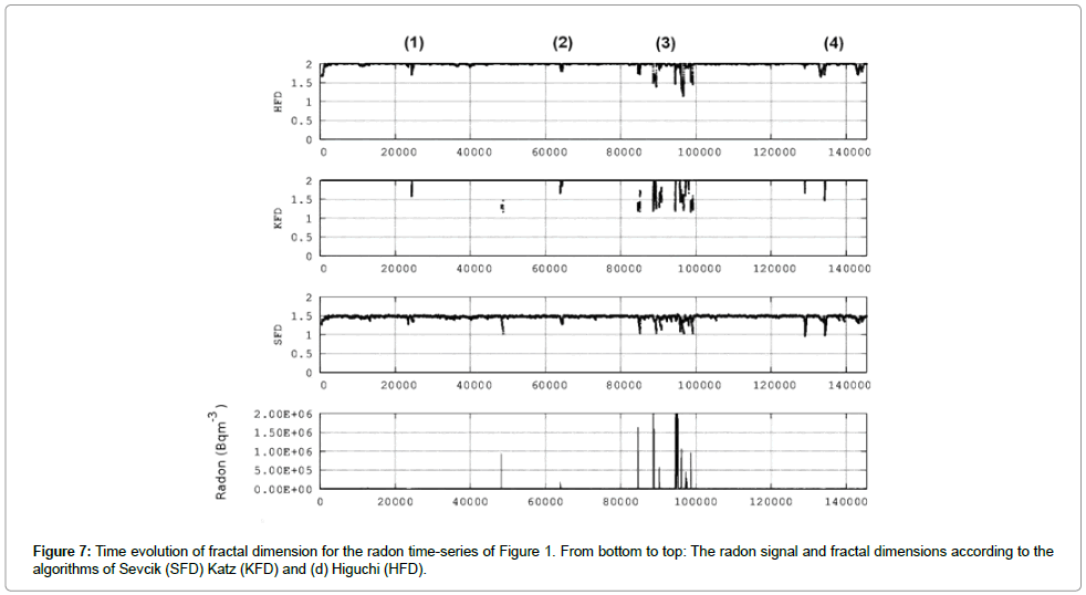
Figure 7: Time evolution of fractal dimension for the radon time-series of Figure 1. From bottom to top: The radon signal and fractal dimensions according to the algorithms of Sevcik (SFD) Katz (KFD) and (d) Higuchi (HFD).
The concept of fractal dimension has been applied with success in processes following the fBm class (the reader ought to emphasize that the fBm systems are more predictable [11,12, 15-17]. For The concept of fractal dimension has been applied with success in processes following the fBm class (the reader ought to emphasize that the fBm systems are more predictable [11,12, 15-17]). For complex fBm systems, the following are valid [32,84-86]: (a) if the system is governed by persistent processes, it exhibits moderate profiles of low fractal dimensions in the range  (b) if anti-persistent processes determine the system's dynamics, the D profiles are rough with values in the range
  (c) if the system is random
  [32]. Under this perspective, the areas (1)-(4) in Figure 7 correspond to persistent underlying dynamics, in contrast to the remaining areas with antipersistent dynamics. Although the results of R/ S analysis indicated mainly mild persistent behavior, still, during these periods, the persistent dynamics were much stronger with R/ S too (H - value peaking, Figure 6, Under this view, the two different techniques provided comparable results. The findings of Figure 5 are closer to those of Figure 7, in the sense that the highly persistent areas were identified in Figure 5, as high b -areas. The results of all the techniques can be compared in terms of the Hurst exponents since these were calculated directly from the R/S analysis and the main parameters of the other techniques can be converted to Hurst exponents by means of linear associations. In specific: Power-law b values can be converted to Hurst exponents from [45]:
b = 2H +1⇒H = 0.5 (b-1), if 1< b = 3 (fBm class) (12a)
and from
b = 2H -1⇒H = 0.5 (b+1), if -1 = b< 1(fGn class) (12b)
DFA exponents a can be converted to Hurst exponents by considering, first, that the association between power-law fractal (b) and DFA (a) exponents is b = 2·a-1 for both the fBm and fGn classes [39,44,47]. Considering the b -H relations of (A), the Hurst exponents can be calculated as:
H = 0.5 [b-1] ⇒H = 0.5[(2a-1)-1]⇒ H = 0.5 [2(a -2) ⇒ H = 0.5 [2 (a-1)]H = a-1 (13a)
for 1< b = 3⇒1< 2 ·a-1 = 3 ⇒2< 2· a = 4⇒1< a = 2 and as
H = 0.5 [b +1]⇒ H = 0.5 [(2a-1) +1] ⇒H = 0.5 (2a)⇒H = a (13b)
for-1 = b < 1-1 = 2 ·a1< 1⇒0 = 2·a< 2⇒0 = a < 1 [39,44,47]. According to the findings of fractal dimension analysis Hurst exponents can be calculated according to the Berry's equation, namely:
H = 2 - D (14)
The following ranges can be observed from (Figures 4-7) regarding the Hurst exponent value range within the corresponding peaks: (a) According to R/S analysis, between 0.7-0.9 and in some -17- segments, between 0.9-1 (Figure 6); (b) According to fractal analysis between 0.6-1 (2.2< b< 3) (Figure 5); (c) According to DFA, the range within the peaks was between 0.2-0.5 (1.2< a < 1.5) (Figure 4); (d) According to fractal dimension analysis, between 0.7-1 (Higuchi method), 0.3-1 (Katz method) and 0-0.5 (Sevcik method). These discrepancies in the Hurst exponent estimation between the different techniques, have been implied in previous publications [27-34,36] and has been discussed extensively [35]. Similar issues have been encountered also in other publications [87,88] and the references therein]. It is, more or less, the simplicity of the linear approach of the equations (12)-(14) that is not fully operating under the actual conditions of measurement. Nevertheless, the overall approach followed in this paper, was not the visual observation of anomalies [2,33-35] nor a delineation through statistical analysis but was rather a holistic approach based on the main processes inside the earth's crust during preparation of earthquakes. The overall approach is in accordance to the findings and interpretations reported in numerous publications [6-41]. Despite that the main event during the period of measurement was medium, the close vicinity to the UALG station, may have been sufficient reason for the reported signs of fractality and long-memory that, importantly, were delineated simultaneously and with separate methods. New data are collected so as to extend this research further and especially in relation to the wellestablished electromagnetic precursors of general failure.
Conclusion
This paper reported time-series data of concentration of radon in soil recorded prior to two earthquakes occurred in Lesvos Island, Greece. The data were derived by a telemetric radon station based on Alpha Guard monitor installed in the University of the Aegean, Lesvos, Greece. A batch of significant radon anomalies was observed during measurement. The data were analyzed through DFA, fractal analysis, R/S analysis and fractal dimension analysis via the Higuchi, Katz and Sevcik methods. The results of the DFA showed four peaks with slopes between 1.2 and 1.5. The fractal analysis method resulted in three peaks with persistent power-law exponent values in the range 2.2 and 3.0. The rescaled-range analysis indicated persistent Hurst exponents between 0.7-0.9 and in some segments, between 0.9-1. The fractal dimension analysis showed four peaks with fractal dimensions in the range 1.3- 2.0 (Higuchi and Katz methods) and 1.0-1.5 (Sevcik method). The results were interpreted in terms of Hurst exponents. Discrepancies in the Hurst exponent estimation between the different techniques were observed. During the radon anomalies and in other segments, significant simultaneous increase in Hurst exponents was detected by all methods. Despite the discrepancies, the relative findings were in agreement for all the methods and provided, in this sense, comparable results. Trends of long-memory were identified and discussed. The findings are compatible with fractal, long-memory and SOC phases of generation of earthquakes.
References
- Hayakawa M, Hobara Y (2010) Current status of seismo-electromagnetics for short-term earthquake prediction. Geomat Nat Haz Risk 1: 115-155.
- Cicerone R, Ebel J, Britton J (2009) A systematic compilation of earthquake precursors. Tectonophysics 476: 371-396.
- Uyeda S, Nagao P, Kamogawa M (2009) Short-term earthquake prediction: current status of seismo electromagnetics. Tectonophysics 470: 205-213
- Shrivastava A (2014) Are pre-seismic ULF electromagnetic emissions considered as a reliable diagnostics for earthquake prediction? Current Science 107: 596-560.
- Khan PA, Tripathi SC, Mansoori AA, Bhawre P, Purohit PK, et al. (2011) Scientific efforts in the direction of successful Earthquake Prediction. International Journal of Geomatics and Geosciences 1: 669-677.
- Cantzos D, Nikolopoulos D, Petraki E, Nomicos C (2015) Identifying long-memory trends in pre-seismic MHz disturbances through support vector machines. J Earth Sci Clim Change 6: 1-9.
- Cantzos D, Nikolopoulos D, Petraki E, Yannakopoulos PH, Nomicos C, et al. (2016) Fractal analysis, information-Theoretic similarities and SVM classification for multichannel, multi-frequency pre-seismic electromagnetic measurements. J Earth Sci Clim Change 7: 1-10.
- Eftaxias K, Kapiris P, Polygiannakis J, Bogris N, Kopanas J, et al. (2001) Signature of pending earthquake from electromagnetic anomalies. Geophys Res Lett 29: 3321-3324.
- Eftaxias K, Kapiris P, Dologlou E, Kopanas J, Bogris N, et al. (2002) EM anomalies before the Kozani earthquake: A study of their behavior through laboratory experiments. Geophys Res Lett 29: 69: 69-4.
- Karamanos K, Dakopoulos D, Aloupis K, Peratzakis A, Athanasopoulou L, et al. (2006) Preseismic electromagnetic signals in terms of complexity. Phys Rev E Stat Nonlin Soft Matter Phys 74: 016104.
- Eftaxias K, Kapiris P, Balasis G, Peratzakis A, Karamanos K, et al. (2006) Unified approach to catastrophic events: From the normal state to geological or biological shock in terms of spectral fractal and non-linear analysis. NHESS 6: 205-228.
- Eftaxias K, Sgrigna V, Chelidze T (2007) Mechanical and EM phenomena accompanying pre-seismic deformation: From laboratory to geophysical scale. Tectonophysics 431: 1-301.
- Eftaxias K, Panin V, Deryugin Y (2007) Evolution-EM signals before earthquakes in terms of meso-mechanics and complexity. Tectonophysics 431: 273-300.
- Eftaxias K, Contoyiannis Y, Balasis G, Kalimeri M, Nikolopoulos S, et al. (2008) Evidence of fractional-Brownian-motion-type asperity model for earthquake generation in candidate pre-seismic electromagnetic emissions. NHESS 8: 657-69.
- Eftaxias K, Athanasopoulou L, Balasis G, Papadimitriou C, Kalimeri M, et al. (2009) Unfolding the procedure of characterizing recorded ultra-low frequency, kHz and MHz electromagnetic anomalies prior to the L’Aquila earthquake as pre-seismic ones -Part 1. NHESS: 1953-1971.
- Eftaxias K, Balasis G, Contoyiannis Y (2010) Unfolding the procedure of characterizing recorded ultra-low frequency, kHZ and MHz electromagnetic anomalies prior to the L’Aquila earthquake as pre-seismic ones - Part 2. NHESS 10: 275-294.
- Eftaxias K (2010) Footprints of non-extensive Tsallis statistics, self-affinity and universality in the preparation of the L'Aquila earthquake hidden in a pre-seismic EM emission. Physica A 389: 133-140.
- Hayakawa M, Ida Y, Gotoh K (2005) Multifractal analysis for the ULF geomagnetic data during the Guam earthquake. Electromagnetic Compatibility and Electromagnetic Ecology, 2005. IEEE 6th International Symposium 24: 239-243.
- Hayakawa M (2007) VLF/LF Radio sounding of ionospheric perturbations associated with earthquakes. Sensors 7: 1141-1158.
- Kalimeri M, Papadimitriou C, Balasis G (2008) Dynamical complexity detection in pre-seismic emissions using non-additive Tsallis entropy. Physica A 387: 1161-1172.
- Kapiris P, Balasis G, Kopanas J, Antonopoulos G, Peratzakis A, et al. (2004) Scaling Similarities of Multiple Fracturing of Solid Materials. Nonlinear Process Geophys 11: 137-151
- Kapiris P, Balasis G, Kopanas J, Antonopoulos G, Peratzakis A, et al. (2004) Scaling Similarities of Multiple Fracturing of Solid Materials. Nonlinear Process Geophys 11: 137-151.
- Kapiris PG, Eftaxias KA, Chelidze TL (2004) Electromagnetic Signature of Prefracture Criticality in Heterogeneous Media. Phys Rev Lett 92: 065702
- Kapiris PG, Eftaxias KA, Nomikos KD, Polygiannakis J, Dologlou E, et al. (2003) Evolving towards a critical point: A possible electromagnetic way in which the critical regime is reached as the rupture approaches. Nonlinear Process Geophys 10: 511-524.
- Kapiris P, Nomicos K, Antonopoulos G, Polygiannakis J (2005) Distinguished seismological and electromagnetic features of the impending global failure: Did the 7/9/1999 M5.9 Athens earthquake come with a warning? Earth Planets Space 57: 215-230.
- Kapiris P, Polygiannakis J, Peratzakis A, Koulouras G, Nomicos C, et al. (2002) VHF-electromagnetic evidence of the underlying pre-seismic critical stage. Earth Planets Space 54: 1237-1246.
- Nikolopoulos D, Petraki E, Marousaki A, Koulouras G, Kottou S, et al. (2012) Environmental monitoring of radon in soil during a very seismically active period occurred in South West Greece. J Environ Monitor 14: 564-578.
- Nikolopoulos D, Petraki E, Vogiannis E, Yannakopoulos PH, Nomicos C, et al. (2014) Traces of self-organisation and long-range memory in variations of environmental radon in soil: Comparative results from monitoring in Lesvos Island and Ileia (Greece). J Radioanal Nucl Chem 299: 203-219.
- Nikolopoulos D, Petraki E, Nomicos C, Yannakopoulos PH, Nomicos C, et al. (2015) Long-Memory Trends in Disturbances of Radon in Soil Prior ML=5.1 Earthquakes of 17 November 2014 Greece. J Earth Sci Clim Change 6: 1-11.
- Nikolopoulos D, Cantzos D, Petraki E, Yannakopoulos PH, Panagiotaras D, et al. (2016) Traces of long-memory in pre-seismic MHz electromagnetic time series-Part 1: Investigation through the R/S analysis and time-evolving spectral fractals. J. Earth Sci Clim Change 7: 1
- Nikolopoulos D, Petraki E, Cantzos D, Panagiotaras D, Koulouras G, et al. (2016) Fractal Analysis of Pre-Seismic Electromagnetic and Radon Precursors: A Systematic Approach J Earth Sci Clim Change 7: 1-11.
- Petraki E, Nikolopoulos D, Fotopoulos A, Panagiotaras D, Nomicos C, et al. (2013) Self- organised critical features in soil radon and MHz electromagnetic disturbances: Results from -22- environmental monitoring in Greece. Appl Radiat Isotopes 72: 39-53.
- Petraki E, Nikolopoulos D, Fotopoulos A, Panagiotaras D, Nomicos C, et al. (2013) Long-range memory patterns in variations of environmental radon in soil. Anal Methods 5: 4010-4020.
- Petraki E, Nikolopoulos D, Nomicos C, Stonham J, Cantzos D, et al. (2015) Fractal analysis of pre-seismic electromagnetic and radon precursors: A systematic approach. J Earth Sci Clim Change 7: 1-11.
- Petraki E, Nikolopoulos D, Nomicos C, Coulouras G, Nomicos C, et al. (2015) Electromagnetic Pre-earthquake Precursors: Mechanisms, Data and Models-A Review. J Earth Sci Clim Change 6: 1-11.
- Petraki E (2016) Electromagnetic radiation and Radon-222 gas emissions as precursors of seismic activity. A Thesis submitted for the Degree of Doctor of Philosophy, Department of Electronic and Computer Engineering.
- Petraki E, Nikolopoulos D, Chaldeos Y (2016) Fractal evolution of MHz electromagnetic signals prior to earthquakes: results collected in Greece during 2009. Geomat Nat Haz Risk 7: 550-564.
- Sarlis N, Skordas E, Varotsos P (2013) Minimum of the order parameter fluctuations of seismicity before major earthquakes in Japan. Proc Natl Acad Sci 110: 13734-738.
- Skordas ES (2014) On the increase of the "non-uniform" scaling of the magnetic field variations before the M(w)9.0 earthquake in Japan. CHAOS 24: 023131
- Smirnova N, Hayakawa M, Gotoh K (2004) Precursory behavior of fractal characteristics of the ULF electromagnetic fields in seismic active zones before strong earthquakes. Phys Chem Earth 29: 445-451.
- Smirnova NA, Hayakawa M (2007) Fractal characteristics of the ground-observed ULF emissions in relation to geomagnetic and seismic activities. J Atmos Sol Terr Phys 69: 1833-1841.
- Surkov V, Uyeda S, Tanaka H, Hayakawa M (2002) Fractal properties of medium and seismoelectric phenomena. Journal of Geodynamics 33: 477-487.
- Nazaroff W, Nero A (1988) Radon and its decay products in indoor air. Wiley, New York, USA.
- Richon P, Bernard P, Labed V (2007) Results of monitoring 222Rn in soil gas of the Gulf of Corinth region, Greece. Rad Meas 42: 87-93
- King CY (1985) Impulsive radon emanation on a creeping segment of the San Andreas fault, California. Pure App Geophys 122: 340-352.
- King CY (1980) Episodic radon changes in Subsurface soil gas along active faults and possible relation to earthquakes. J Geophys Res 85: 3065-3078.
- Al-Tamimi MH, Abumura KM (2001) Radon anomalies along faults in North of Jordan. Rad Meas 34: 397-400
- Tansi C, Tallarico A, Iovine G, Gallo MF, Falcone G (2005) Interpretation of radon anomalies in seismotectonic and tectonic-gravitational settings: the south-eastern Crati graben (Northern Calabria, Italy). Tectonophys 396: 181-193.
- Walia V, Yang T, Hong W, Lin S, Fu C, et al. (2009) Geochemical variation of soil–gas composition for fault trace and earthquake precursory studies along the Hsincheng fault in NW Taiwan. App Rad Isotop 67: 1855-1863.
- Whitehead NE, Barry BJ, Ditchburn RG (2007) Systematics of radon at the Wairakei geothermal region, New Zealand. J Env Rad 92: 16-29.
- Zafrir H, Steinitz G, Malik U, Haquin G, Gazit-Yaari N (2009) Response of Radon in a seismic calibration explosion, Israel. Rad Meas 44: 193-198.
- Erees F, Aytas S, Sac M, Yener G, Salk M (2007) Radon concentrations in thermal waters related to seismic events along faults in the Denizli Basin, Western Turkey. Rad Meas 42: 80-86.
- Choubey V, Kumar N, Arora B (2009) Precursory signatures in the radon and geohydrological borehole data for M4.9 Kharsali earthquake of Garhwal Himalaya. Sci Total Environ 407: 5877-5883.
- Mogro-Campero A, Fleischer R (1979) Search for long-distance migration of subsurface radon. US Department of Energy, Washington D.C. USA.
- Ghosh D, Deb A, Dutta S (2012) Multifractality of radon concentration fluctuation in earthquake related signal. Fractals 20: 33-39
- Genitron (1994) Alpha guard PQ2000/MC50, multiparameter radon monitor. Genitron Instruments Ltd, Frankfurt, Germany.
- Louizi, A, Nikolopoulos D, Koukouliou V (2003) Study of a Greek area with enhanced radon concentrations. Rad Prot Dosim 106: 219-226.
- Hurst H, Black R, Simaiki Y (1965) Long-term storage: An experimental study. Constable, London, UK.
- Hurst HE (1951) Long-term storage capacity of reservoirs. Trans Am Soc Civ Eng 116: 770-799.
- Mandelbrot BB, Wallis JR (1969) Some long-range properties of geophysical records. Water Re-sources Res. 5: 321.
- Stratonovich RL (1981) Topics in the theory of random noise. Gordon and Breach. New York, USA.
- Peng C, Buldyrev S, Goldberger A, Havlin S, Sciortino F, et al. (1992) Long-range correlations in nucleotide sequences. Lett Nature 356: 168-170.
- Peng CK, Mietus JE, Hausdor JM, Havlin S, Stanley HE, et al. (1993) Magnitude and sign correla-tions in heartbeat fluctuations. Phys Rev Lett 70: 1343-1346.
- Peng CK, Buldyrev SV, Havlin S, Simons M, Stanley HE, et al. (1994) Mosaic organization of DNA nucleotides. Phys Rev E 49: 1685-1689.
- Peng CK, Havlin S, Stanley HE (1995) Quantification of scaling exponents and crossover phenomena in nonstationary heartbeat time series. Chaos 5: 82-87.
- Buldyrev S, Goldberger A, Havlin S, Manligna R, Matsa M, et al. (1995) Long-range correlation properties of coding and noncoding DNA sequences: GenBank analysis. Phys Rev E Stat Phy Plasmas Fluids Relat. Interdiscip Topics 51: 5084-5091.
- Peng CK, Hausdorff JM, Havlin S, Mietus JE, Stanley HE, et al. (1998) Multiple-time scales analysis of physiological time series under neural control. Phys A 249: 491-500.
- Hu K, Ivanov PC, Chen Z (2001) Effect of trends on detrended fluctuation analysis. Phys Rev E Stat Nonlin Soft Matter Phys 64: 011114.
- Chen Z, Ivanov PC, Hu K (2002) Effect of non-stationarities on detrended fluctuation analysis. Phys Rev E 65: 1–15 041107.
- Telesca L, Lasaponara R (2006) Vegetational patterns in burned and unburned areas investi- gated by using the detrended fluctuation analysis. Phys A 368: 531-535.
- Ivanova K, Ausloos M (1999) Application of the detrended fluctuation analysis (DFA) method for describing cloud breaking. Physica A 274: 349-354.
- Koscielny-Bunde E, Bunde A, Havlin S (1998) Indication of a universal persistence law governing atmospheric variability. Phys Rev Lett 81: 25 .
- Vandewalle N, Ausloos M (1997) Coherent and random sequences in financial fluctuations. Physica A 246: 454-459.
- Ivanov PC, Rosenblum MG, Peng CK (1999) Multifractality in human heartbeat dynamics. Nature 399: 461-465.
- Lopez T, Martinez-Gonzalez C, Manjarrez J (2009) Fractal analysis of EEG Signals in the brain of epileptic rats, with and without biocompatible implanted neuroreservoirs. AMM 15: 127-136.
- Gilmore M, Yu C, Rhodes T (2002) Investigation of rescaled range analysis, the Hurst exponent, and long-time correlations in plasma turbulence. Phys Plasmas 9: 1312-1317.
- Kilcik A, Anderson C, Rozelot J (2009) Non-linear prediction of solar cycle 24. Astrophys J 693: 1173-1177.
- Rehman S, Siddiqi A (2009) Wavelet based Hurst exponent and fractal dimensional analysis of Saudi climatic dynamics. Chaos Solitons Fractals 39: 1081-1090.
- Granero MS, Segovia JT, Perez JG (2008) Some comments on Hurst exponent and the long memory processes on capital markets. Physica A 387: 5543–5551.
- Dattatreya G (2005) Hurst parameter estimation from noisy observations of data traffic traces. Paper presented at the 4th WSEAS International Conference on Electronics, Control and Signal Processing 193: 198.
- Li X, Polygiannakis J, Kapiris P (2005) Fractal spectral analysis of pre-epileptic seizures in terms of criticality. J Neural Eng 2: 11-6.
- Higuchi T (1988) Approach to an irregular time series on the basis of the fractal theory. Physica D 31: 277-283.
- Katz MJ (1988) Fractals and the analysis of waveforms. Comp Biol Med 18: 145-156.
- Sevcik C (2010) A procedure to estimate the fractal dimension of waveforms. ArXiV 1003: 5266.
- Bascompte J, Vilaa C (1997) Fractals and search paths in mammals. Landsc Ecol 12: 213-221
- Katz M, George E (1985) Fractals and the analysis of growth paths. Bull Math Biol 47: 273-286
- Mortimer S, Swan M, Mortimer D (1996) Fractal analysis of capacitating human spermatozoa. Hum Reprod 11: 1049-1054.
- Morgounov V (2001) Relaxation creep model of impending earthquake. Ann Geophys 44: 369-381.
Citation: Nikolopoulos D, Matsoukas C, Yannakopoulos P, Petraki E, Cantzos D, et al. (2018) Long-Memory and Fractal Trends in Variations of Environmental Radon in Soil: Results from Measurements in Lesvos Island in Greece. J Earth Sci Clim Change 9:460. DOI: 10.4172/2157-7617.1000460
Copyright: © 2018 Nikolopoulos D, et al. This is an open-access article distributed under the terms of the Creative Commons Attribution License, which permits unrestricted use, distribution, and reproduction in any medium, provided the original author and source are credited.
Select your language of interest to view the total content in your interested language
Share This Article
Recommended Journals
Open Access Journals
Article Tools
Article Usage
- Total views: 5660
- [From(publication date): 0-2018 - Nov 15, 2025]
- Breakdown by view type
- HTML page views: 4611
- PDF downloads: 1049