Multi-model Climate Change Projections for Belu River Basin, Myanmarunder Representative Concentration Pathways
Received: 09-Nov-2015 / Accepted Date: 14-Dec-2015 / Published Date: 20-Dec-2015 DOI: 10.4172/2157-7617.1000323
Abstract
Climate change impacts and adaptation related studies in Myanmar are scanty. Therefore this study aims to project future climate scenarios considering two key meteorological parameters-temperature and precipitation -in Belu River Basin in Myanmar. Multi-GCMs approach with ten different GCMs on 10th to 90th percentile uncertainty range is studied using time series data of nine meteorological stations. Quantile mapping technique is used to correct the bias in raw GCM data. Bias corrected GCM ensembles are analysed for a wide range of climate scenarios to get the complete picture of climate change pattern for 21st century. All ten GCM ensembles (four RCP scenarios) indicate that the monsoon to get wetter as well as delayed. August will witness highest amount of rainfall. More rain concentrating over shorter time span suggests likely increase in extreme precipitation events. Only a slight increase is expected on the overall annual precipitation (-1.78~+ 9.14%, range of values from four scenarios). Minimum temperature is found to increase almost twice (+0.64~+5.27C) as compared to maximum temperature (+0.56~+2.82°C) under different scenarios. Summer is the hardest hit season with May and April the most affected months for maximum and minimum temperatures respectively. These results are very useful for further research on assessment of vulnerability and adaptation on water resources and water use sectors in Belu River Basin in Myanmar.
Keywords: Climate change; Multi-GCM; RCP scenarios; Temperature; Precipitation; Belu River Basin; Myanmar
10468Introduction
Global climate models, also known as general circulation models (GCMs), are models which generate the meteorological variables such as precipitation (rainfall), temperature, wind speed, relative humidity, solar radiation etc. These meteorological variables are generated by solving the primitive equations of thermodynamics, mass and momentum [1]. Climatic statistics are obtained as the time series future data for different Green House Gas (GHG) emission scenarios. However, climate variables simulated by individual GCMs often do not agree with observed time series. In order to create climatic statistics, the GCMs are usually used as a multi-model analysis [2]. With the lead of Intergovernmental Panel on Climate Change (IPCC), several institutes and organizations researched on climate change impact with respect to various climate variables and resulted as GCM gridded data in various resolutions ranging from 100 to 300 km grid size. This study involves multi-GCMs approach of analysis (ensemble generation) with ten different GCMs from Infrastructure for the European Network for Earth System Modelling (IS-ESNE) portal for three meteorological variables viz. precipitation, maximum temperature and minimum temperature for Belu River Basin of Myanmar.
Due to systematic and random model errors, however, GCM simulations often show considerable deviations from observations. To be able to simulate most reliable result, bias correction and downscaling with observed ground data is required. There are several methods to downscale the climate variables from the general circulation model [3,4]. These correction approaches can be classified according to their degree of complexity ranging from simple methods such as delta change approach to more advanced methods such as quantile mapping. The bias correction methods are used to identify the bias-possible differences between observed and simulated climate variables. This bias relation values are then used to correct both control and scenario GCM runs with a transformation algorithm [5].
Daily ground stations record of precipitation and temperature and daily GCM simulated hindcast, from 1976to 2005 (30 years), are used for the bias correction process. The future projections for three periods are defined as 2020s (early period, from 2010 to 2039), 2050s (middle period, from 2040 to 2069) and 2080s (late period, from 2070 to 2099) for analysis under different Representative Concentration Pathways (RCPs) scenarios.
The projected climate change scenarios are associated with large uncertainties. For water resource management, these projection uncertainties importantly contribute to the total uncertainty, in addition to factors such as natural variability and changes in water demand [6]. The climate change impact projections for water management and planning purposes has been done by several studies and at the same time it has also became the particular interest in the quantification of uncertainties [7]. The variability is considered to be indicated by the range between the 10th and the 90th percentile values, following similar studies [8,9]. The IPCC Fifth Assessment Report (AR5) defines four Representative Concentration Pathways (RCPs) depending on how much greenhouse gases are possibly emitted in the years to come such as RCP 2.6, RCP 4.5, RCP 6.0, and RCP 8.5 which are named for a possible range of radiative forcing values in the year 2100 relative to pre-industrial values (+2.6, +4.5, +6.0, and +8.5 W/m2, respectively). As Belu River Basin is still under development, there are several possibility for its future social and industrial development trend. Since this trend can range from gradual development to high speed growth into industrialized city, all four RCPs scenario shave been considered to know the complete picture of possible climate change over coming century. The catchment of the study area covers the natural Inle lake, Mobye reservoir and three hydropower stations at downstream. The major objectives of this study are to investigate the future spatial and temporal changes in temperature and rainfall in Belu River Basin and to investigate the climate uncertainty range and the reliability of GCMs on the study area.
Methodology
Study area
The study area, Belu River Basin, falls under two states of Myanmar namely Shan and Kayar states (Figure 1). With a total area of 8,329.11 km2 the basin is located between 96º31´41"E-97º25´31" E longitudes and 19º23´ 31" N-21º12´31" N latitudes. The basin includes Inle lake and Mobye reservoir from where the water flows as Belu River which in turn merges with Salween river (Thanlwin river) at the downstream of the basin. The basin has an annual average rainfall of 1,273 mm/yr. Around 3/4th of land use is dominated by forest cover (42.57%) and agricultural pastures (33.68%) while the rest constitutes shrub, water bodies and urban areas.
The Inle lake comprise the cultural and national heritage of 35 floating villages and floating plantation fields. This area is also the largest tomato plantation fields in Myanmar which has average production of 50 tons/day [10]. The first hydropower project of Myanmar, Lawpita No. 2 (168 MW), is also located in the basin in conjunction with other two cascade hydropower stations -Lawpita No.1 (28 MW) and Lawpita No. 3 (48 MW). The multipurpose Mobye reservoir (827 MCM) is utilized for irrigation, hydropower generation and water supply for the Loikaw city at the downstream of dam.
Increase in floods and droughts problem in recent times come as a sign of climate change impact in the basin. In 1998 and 1999, the storage of the Mobye reservoir was depleted due to low rainfall. In 2011, Inle lake shrunk down to 70 km2 which was less than half (163 km2) of the area it covered three years ago. The change was attributed to climate change and excessive sedimentation. Water released from the Mobye Dam into the Belu River, along with heavy August rains, caused flooding in the lowlands of Loikaw, affecting more than 1,129 households and destroying 150 acres of rice fields [10].
There is no doubt that the Belu River Basin has a multi-faceted people-economy-water interlinkage. This link is highly vulnerable to hydro-meteorological changes as observed specially in recent past. Sustainability of all aspects and the basin as a whole thus mandates climate change impact study in the region.
Data description
There are three types of data used in this study (Table 1a) the historical observed daily data (maximum/minimum temperature and precipitation), b) the global datasets available in public domain, and c) General Circulation Model (GCM) datasets. The observed data were collected from the Department of Meteorology and Hydrology, Ministry of Electricity and Irrigation Department of Myanmar. The dataset consists of nine rain gauge stations out of which six stations include temperature record as well. From these stations the daily records spanning over 1976-2005 (30 years) are used for climate change study. Four out of nine rain stations and two of out of six temperature stations exhibited data continuity issues ranging from data gap of few months to partial period of data. Widely used global datasets (APHRODITE, Princeton, and Santa Clara) were utilized to assess and solve these data continuity issues using linear regression method. Incorporation of all the observed stations meant that the spatial variability of climate was being addressed more effectively. For future climatic projections, a total of ten GCMs were selected based on the availability of RCP scenarios and fineness of spatial resolution.
| Observed data | |||||||||||||
|---|---|---|---|---|---|---|---|---|---|---|---|---|---|
| SN | Station | Data Continuity | Annual Rainfall (mm/yr.) | Tmax(°C) | Tmean(°C) | Tmin(°C) | |||||||
| 1 | Heho | 1976 - 2005 | 1,002 | 27.05 | 20.23 | 13.41 | |||||||
| 2 | Lawpita | 1981 - 1989 | 1,098 | - | - | - | |||||||
| 3 | Loikaw | 1976 - 2005 | 1,009 | 28.86 | 22.76 | 16.66 | |||||||
| 4 | Loilem | 1976 - 2005 | 1,338 | 25.81 | 19.03 | 12.25 | |||||||
| 5 | Mobye | 1976 - 1991 | 964 | - | - | - | |||||||
| 6 | Namsang | 1996 - 2005 | 1,442 | 29.04 | 21.68 | 14.32 | |||||||
| 7 | Pekon | 1987 - 2005 | 909 | - | - | - | |||||||
| 8 | Pinlaung | 1976 - 2005 | 1,972 | 23.96 | 18.24 | 12.53 | |||||||
| 9 | Taunggyi | 1976 - 2005 | 1,513 | 24.85 | 19.53 | 14.2 | |||||||
| Global Datasets | |||||||||||||
| SN | Name | Source/Developer/Research Institute | Resolution | Source Web Link | |||||||||
| Long. by Lat. | |||||||||||||
| 1 | APHRODITE | National Center for Atmospheric Research (NCAR), University Corporation for Atmospheric Research (UCAR) | 0.25° × 0.25° | https://climatedataguide.ucar.edu/climate-data/aphrodite-asian-precipitation-highly-resolved-observational-data-integration-towards | |||||||||
| 2 | Princeton | Princeton University | 0.25° × 0.25° | http://hydrology.princeton.edu/home.php | |||||||||
| 3 | Santa Clara | Santa Clara University | 0.50° × 0.50° | http://www.engr.scu.edu/~emaurer/global_data | |||||||||
| GCM Datasets | |||||||||||||
| SN | Name | Developer/Research Institute | Resolution | RCP | RCP | RCP | RCP | ||||||
| Long. × Lat. | 2.6 | 4.5 | 6 | 8.5 | |||||||||
| 1 | BCC-CSM1.1 | Beijing Climate Center (BCC) and ChinaMeteorological Administration (CMA), based on NCAR CCSM2.0.1, China | 2.8125° × 2.8125° | √ | √ | √ | √ | ||||||
| 2 | BNU-ESM | Beijing Normal University, China | 2.8125° × 4.0909° | √ | √ | √ | |||||||
| 3 | CanESM2 | Canadian Centre for Climate Modelling and Analysis, Canada | 2.8125° × 2.8125° | √ | √ | √ | |||||||
| 4 | CCSM4 | National Center for Atmospheric Research (NCAR), USA | 1.25° × 0.9375° | √ | √ | √ | √ | ||||||
| 5 | GFDL-CM3 | Geophysical Fluid Dynamics Laboratory, USA | 2.5° × 2.0° | √ | √ | √ | √ | ||||||
| 6 | IPSL-CM5A-MR | Institut Pierre-Simon Laplace, France | 2.5° × 1.2587° | √ | √ | √ | √ | ||||||
| 7 | MIROC-ESM | Japan Agency for Marine-Earth Science and Technology, Atmosphere and Ocean Research Institute (The University of Tokyo), Japan | 2.8125° × 2.8125° | √ | √ | √ | √ | ||||||
| 8 | MIROC5 | Atmosphere and Ocean Research Institute, University of Tokyo, Japan | 1.4063° × 1.4063° | √ | √ | √ | √ | ||||||
| 9 | MPI-ESM-MR | Max Planck Institute for Meteorology (MPI-M), Germany | 1.875° × 1.875° | √ | √ | √ | |||||||
| 10 | MRI-CGCM3 | Meteorological Research Institute, Japan | 1.125° × 1.125° | √ | √ | √ | √ | ||||||
Table 1: Data used in the study.
Climate of the basin
Myanmar has three seasons-summer (March-May), monsoon (June-October) and winter (November-February). However in the study region, monsoon usually starts a bit earlier (mid or end of May). Usually August is the wettest month receiving 235 mm rainfall on average. The average annual rainfall and temperature of the observed stations for the study period are as shown in Table 1. The Southern/ downstream parts of the basin are drier in terms of rainfall (Figure 1 and Table 1) while the Northern/upstream parts are relatively wetter (Namsang, Loilem, Taunggyi, Heho and Pinlaung).The highest annual average rainfall is found around the middle portion of the basin (Pinlaung-1,973 mm/yr.). The average mean temperature over the basin ranges from 18.24 to 22.76°C. Namsang station has the highest average annual maximum temperature (29.04°C). From the records, 1998 was the hottest year when the temperature increased up to 30.44°C at Loikaw station and 30.07°C at Namsang station. Generally, April is the hottest month while December is the coldest with temperatures that sometimes plunge down to subzero values.
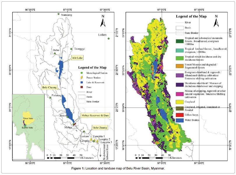
Figure 1: Location and landuse map of Belu River Basin, Myanmar.
Data continuity: linear regression using global datasets
Arguably the most commonly observed problem in precipitation and temperature data is missing observations/readings. Spatial networks such as global dataset are used in some cases to provide supplementary climate data [11]. However, it is essential to check the performance of these data before application. Some of the most widely use global datasets for tackling data continuity issues are -APHRODITE, Princeton and Santa Clara [9,12,13]. The agreement between the stations with complete observed data and global data is checked statistically using coefficient of determination, a widely applied performance statistics in the climate studies. The best match global data set is then used to simulate time series for data continuity. The simulation is carried out using linear regression method which is the most simple and commonly used method in climate studies [12].
Climate change projection using multi-GCM approach
It has been noticed that there is a large spread in the GCM projections and it is especially true for precipitation in the Asian region [9,14]. Thus there is a higher level of uncertainty while working with GCM projections. Three of the main sources of this uncertainty are: a) model uncertainty due to the structural differences among GCMs, b) scenarios uncertainty due to different radiative forcing, and c) uncertainty due to the natural climate variability. There is growing agreement in considering the climate impact study by an ensemble of GCMs outputs. Accordingly, this study embraces multi-GCMs approach with multi-scenarios climate pattern analysis. A total of ten GCMs have been considered based on the priority of data availability for all four RCP scenarios (IN-ENSE) and the fineness of spatial resolution (Table 1).
Bias correction-quantile mapping
Till date researchers working on climate change impact study have applied several bias correction methods for de-biasing GCM data. Some have even performed comparative study of effectiveness and reliability among these methods. All conclude that quantile mapping (also widely mentioned in literature as probability mapping, statistical downscaling, or histogram equalization) is the method that generates optimized best result [15-17]. Moreover, quantile mapping has several advantages over other methods such as: 1) corrects mean, standard deviation (variance), wet-day frequencies and intensities, 2) events are adjusted non-linearly, and 3) variability of corrected data is more consistent with original data [17,18].
In quantile mapping, a function h is determined that maps a modeled variable Pm such that its new distribution equals the distribution of the observed variable Po through statistical transformations. Following Piani et al., [19], the transformations can be denoted by the following formula –
 (1)
(1)
Quantile mapping is an application of the probability integral transform. If the distribution of the variable of interested is known, Gudmundsson et al. [18] explained that the transformation h is defined as:
 (2)
(2)
Where Fm represents cumulative distribution function of modelled parameter Pm and Fo−1 represents the inverse cumulative distribution function (or quantile function) corresponding to observed parameter Po. Thus quantile mapping adjusts the distribution of a modeled parameter (Pm) to match the distribution of an observed parameter (Po) using distribution derived transformations.
In this study Quantile mapping was carried out in R language [20] using qmap package, which is available on the Comprehensive R Archive Network. The package estimates the values of the quantilequantile relation of observed and modelled data for regularly spaced quantiles using local linear least square regression and performs quantile mapping by interpolating the empirical quantiles. The corresponding values of the quantiles of observe is estimated using local linear least squares regression. For each quantile of modelled data, nearest data points is plotted to fit a local regression line to estimate value of the quantile of observed data [21]
Improvement in agreement between observed data and GCM hindcast data was assessed statistically in order to conclude on the performance of the quantile mapping method of bias correction. Widely used statistical parameters-standard deviation (σ), correlation (r) and root mean square error (RMSE) were used to check performance of the model. The models exhibiting high correlation, small root mean square error and a standard deviation close to that of the observed data were considered suitable to apply for the study area [22,23].
Results and Discussions
Global datasets for data continuity
It was seen that for precipitation APHRODITE is the most reliable alternative while for temperature all three options were consistent (Table 2). However, since APHRODITE temperature dataset lacks daily extreme values (only daily average available), Santa Clara data is used for simulation of maximum and minimum temperature. Results of the simulations are also tabulated in Table 2.
| Precipitation | ||||||||||||||||||||||
|---|---|---|---|---|---|---|---|---|---|---|---|---|---|---|---|---|---|---|---|---|---|---|
| Stations with complete data vs global datasets (1976-2005) | Stations with partial data: before and after simulation | |||||||||||||||||||||
| Name | Aphrodite | Princeton | Santa Clara | Name | Before simulation | After simulation 1976-2005 | ||||||||||||||||
| Observed period | Aphrodite | Princeton | Santa Clara | |||||||||||||||||||
| Heho | 0.719 | 0.554 | 0.565 | Lawpita | 1981-1989 | 0.719 | 0.639 | 0.505 | 0.831 | |||||||||||||
| Loikaw | 0.888 | 0.642 | 0.64 | Mobye | 1976-1991 | 0.73 | 0.664 | 0.618 | 0.78 | |||||||||||||
| Loilem | 0.8 | 0.626 | 0.622 | Namsang | 1996-2005 | 0.587 | 0.721 | 0.634 | 0.852 | |||||||||||||
| Pinlaung | 0.703 | 0.688 | 0.592 | Pekon | 1987-2005 | 0.599 | 0.477 | 0.556 | 0.724 | |||||||||||||
| Taunggyi | 0.867 | 0.667 | 0.727 | |||||||||||||||||||
| Maximum and Minimum Temperature | ||||||||||||||||||||||
| Stations with complete data vs global datasets (1976-2005) | Stations with partial data: before and after simulation | |||||||||||||||||||||
| Name | Aphrodite | Princeton | Santa Clara | Name | Before simulation | After simulation 1975-2005 | ||||||||||||||||
| Observed Period | Aphrodite | Princeton | Santa Clara | |||||||||||||||||||
| Loikaw | Max | 0.989 (Avg) | 0.835 | 0.894 | Heho | Max | 1980-2005 | 0.919 (Avg) | 0.828 | 0.863 | 0.882 | |||||||||||
| Min | 0.949 | 0.954 | Min | 1980-2005 | 0.94 | 0.938 | 0.948 | |||||||||||||||
| Loilem | Max | 0.919 (Avg) | 0.843 | 0.839 | Namsang | Max | 1996-2005 | 0.931 (Avg) | 0.821 | 0.767 | 0.956 | |||||||||||
| Min | 0.894 | 0.876 | Min | 1996-2005 | 0.924 | 0.931 | 0.988 | |||||||||||||||
| Pinlaung | Max | 0.894 (Avg) | 0.748 | 0.745 | ||||||||||||||||||
| Min | 0.931 | 0.937 | R2 with selected global source (partial period) | |||||||||||||||||||
| Taunggyi | Max | 0.970 (Avg) | 0.84 | 0.87 | R2 with selected global source (complete period) | |||||||||||||||||
| Min | 0.952 | 0.965 | ||||||||||||||||||||
Table 2: Comparative analysis on coefficient of determination (R2) of global data and ground observations; performance evaluation of linear regression as a method for augmenting data continuity.
Performance evaluation of quantile mapping
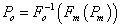
The quantile mapping method of bias correction was found to have relatively increased the agreement between the GCM hindcast series with the observed data. Table 3 shows that all three climatic parameters improved considerably after de-biasing via quantile mapping. Multi- GCM results of bias correction for a couple of stations have been presented as Taylor diagrams [22,23] in Figure 2. In a Taylor diagram, solid line represents standard deviation of the observed data, x-axis represents perfect correlation and the circle on the x-axis represents zero RMSE point. Hence, closeness to the solid line, the x-axis and the circle on x-axis are traits of good/improved GCM dataset.
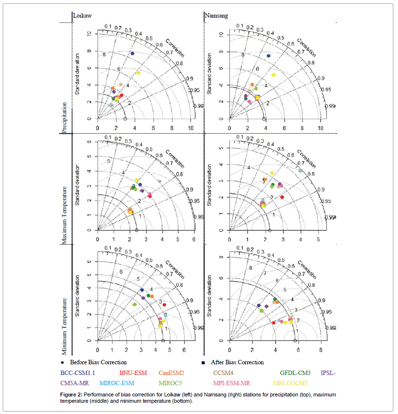
Figure 2: Performance of bias correction for Loikaw (left) and Namsang (right) stations for precipitation (top), maximum temperature (middle) and minimum temperature (bottom).
| Variable | Evaluation indices | Before Correction | After Correction |
|---|---|---|---|
| Precipitation | r | 0.47 - 0.71 | 0.61 - 0.80 |
| σ διφφερενχε | 0.929 (avg.) | 0.136 (avg.) | |
| RMSE (mm) | 3.94 - 4.98 | 2.27 - 3.84 | |
| Maximum Temperature | r | 0.56 - 0.70 | 0.75 - 0.85 |
| σ διφφερενχε | 1.609 (avg.) | 0.030 (avg.) | |
| RMSE (°C) | 3.28 - 6.11 | 1.31 - 1.61 | |
| Minimum Temperature | r | 0.78 - 0.81 | 0.92 - 0.96 |
| σ διφφερενχε | 0.052 (avg.) | 0.010 (avg.) | |
| RMSE (°C) | 3.21 - 6.21 | 1.18 - 2.04 |
Table 3: Results of bias correction-range of evaluation indices amongst GCMs.
Uncertainty analysis
Deriving GCM ensemble (average results of all model projections considered) for each scenario, uncertainty analysis was carried out by studying the distribution of projected data. Seven GCMs were used to derive the ensemble for RCP 6.0 scenario due to unavailability of the scenario run from all GCMs. As per previous literature, distribution range from 10th to 90th percentile is considered as future climate change projection for the study area. The results of uncertainty analysis of GCMs’ annual average values at Loikaw station for all future time periods are shown in Figure 3.
Figure 3: Climate uncertainty for future periods for all RCP scenarios at Loikaw station (i) precipitation (ii) maximum temperature and (iii) minimum temperature.
Sensitivity and reliability of GCMs
In multi-GCMs climate model application such as this, the general impact of GCM models on the climate change projection should be analyzed. Upon analysis it is found that the pattern and trend of the GCM models usually follow that of the monthly median values while that their intensity varies. The early period (2020s) of RCP 2.6, which shows clear variations among GCM runs, is selected to analyze the stability and sensitivity of the GCMs (Figure 4). For precipitation, August and October are considered more sensitive as there are more deviations of GCMs during these period, but however for temperature month of April doesn’t show much deviation between GCMs but months of January and February shows more deviation. The CCSM4 and BCC-CSM1.1 models are usually seen to simulate greater peak rainfall in the basin while GFDL-CM3 model gives an increase in minimum temperature during monsoon period. However, uncertainty ranges such as these due to few GCMs have no major impact on the overall median of GCM ensemble. This proves that multi-GCMs approach is a better option in terms of enhancing reliability and accuracy of results compared to utilization of a single or few GCMs.
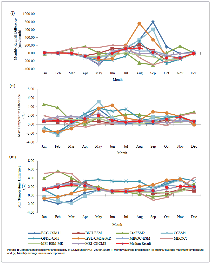
Figure 4: Comparison of sensitivity and reliability of GCMs under RCP 2.6 for 2020s (i) Monthly average precipitation (ii) Monthly average maximum temperature and (iii) Monthly average minimum temperature.
| 4a: Precipitation (mm) | |||||||||||||
|---|---|---|---|---|---|---|---|---|---|---|---|---|---|
| Month | Baseline | RCP 2.6 | RCP 4.5 | RCP 6.0 | RCP 8.5 | ||||||||
| 2020s | 2050s | 2080s | 2020s | 2050s | 2080s | 2020s | 2050s | 2080s | 2020s | 2050s | 2080s | ||
| Jan | 3.78 | 4.24 | 3.81 | 4.29 | 3.29 | 4.89 | 4.14 | 3.71 | 4.34 | 4.91 | 3.77 | 3.78 | 3.42 |
| Feb | 5.42 | 8.62 | 7.81 | 9.43 | 7.4 | 8.7 | 12.28 | 6.05 | 7.44 | 7.47 | 8.12 | 9.01 | 8.7 |
| Mar | 8.11 | 8.53 | 12.83 | 16.13 | 9.52 | 14.52 | 16.46 | 2.87 | 4.33 | 12.31 | 10.85 | 12.8 | 16.02 |
| Apr | 45.13 | -0.11 | 4.26 | 10.24 | -0.76 | 6.61 | 13.52 | -7.34 | 0.48 | 5.89 | 2.14 | 9.26 | 17.95 |
| May | 157.97 | -60.39 | -44.66 | -29.86 | -52.86 | -39.52 | -11.76 | -82.22 | -52.73 | -32.16 | -58.23 | -30.97 | -11.77 |
| Jun | 199.02 | -64.13 | -52.88 | -34.98 | -61.93 | -42.6 | -25.64 | -72.64 | -40.4 | -20.99 | -59.95 | -31.83 | -22.49 |
| Jul | 207.82 | -5.2 | 15.68 | 12.74 | -7.41 | 17.87 | 13.12 | -4.97 | 24.74 | 43.81 | 0.26 | 36.61 | 41.04 |
| Aug | 234.69 | 22.29 | 21.02 | -7.89 | 27.05 | 31.39 | 13.49 | 44.24 | 54.53 | 43.75 | 28.33 | 38.96 | 37 |
| Sep | 210.47 | 25.31 | -5.91 | -37.77 | 37.7 | 1.13 | -23.27 | 47.14 | 4.57 | -17.74 | 22.92 | 13.23 | -8.04 |
| Oct | 131.09 | 13.55 | 7.92 | -7.65 | 17.65 | 15.62 | -1.51 | 32.44 | 11.47 | 2.62 | 14.39 | 6.47 | -4.31 |
| Nov | 58.84 | 36.76 | 37.71 | 32.86 | 32.58 | 33.5 | 34.99 | 30.81 | 38.8 | 28.57 | 42.78 | 33.5 | 30.57 |
| Dec | 10.9 | 11.17 | 9.6 | 9.81 | 11.13 | 8.91 | 12.18 | 14.46 | 10.47 | 8.19 | 9.96 | 10.36 | 8.26 |
| 4b: Maximum Temperature (°C) | |||||||||||||
| Month | Baseline | RCP 2.6 | RCP 4.5 | RCP 6.0 | RCP 8.5 | ||||||||
| 2020s | 2050s | 2080s | 2020s | 2050s | 2080s | 2020s | 2050s | 2080s | 2020s | 2050s | 2080s | ||
| Jan | 24.53 | -0.17 | 0.45 | 1.04 | -0.14 | 0.73 | 1.49 | -0.94 | -0.25 | 0.68 | -0.14 | 1.04 | 2.56 |
| Feb | 26.5 | -0.77 | 0.2 | 0.9 | -0.54 | 0.39 | 1.46 | -1.49 | -0.68 | 0.51 | -0.67 | 0.78 | 2.59 |
| Mar | 29.31 | 0.01 | 0.61 | 0.84 | 0.03 | 0.68 | 1.13 | -0.53 | 0.32 | 0.97 | 0 | 1.04 | 2.57 |
| Apr | 30.75 | 0.91 | 1.11 | 1.09 | 0.89 | 1.31 | 1.38 | 0.83 | 1.16 | 1.57 | 0.83 | 1.58 | 2.43 |
| May | 28.54 | 2.28 | 2.4 | 2.1 | 2.36 | 2.56 | 2.32 | 2.83 | 2.81 | 2.91 | 2.37 | 3.01 | 4 |
| Jun | 26.17 | 1.3 | 1.4 | 1.22 | 1.37 | 1.67 | 1.82 | 1.5 | 1.61 | 2.24 | 1.43 | 2.08 | 3.2 |
| Jul | 25.49 | 0.85 | 0.96 | 1.02 | 0.71 | 1.3 | 1.63 | 0.65 | 1.09 | 1.74 | 0.73 | 1.64 | 2.77 |
| Aug | 25.5 | 0.51 | 0.78 | 0.94 | 0.47 | 1.11 | 1.5 | 0.36 | 0.94 | 1.63 | 0.53 | 1.47 | 2.65 |
| Sep | 26.34 | 0.89 | 1.07 | 0.9 | 0.74 | 1.24 | 1.31 | 0.81 | 1.26 | 1.71 | 0.83 | 1.6 | 2.47 |
| Oct | 26.41 | 1.09 | 1.08 | 1 | 1.04 | 1.38 | 1.32 | 1.09 | 1.59 | 1.73 | 1.12 | 1.74 | 2.32 |
| Nov | 25.11 | 1.3 | 1.36 | 1.27 | 1.37 | 1.62 | 1.82 | 1.35 | 1.58 | 2.03 | 1.28 | 2.14 | 3.05 |
| Dec | 23.88 | 0.44 | 0.93 | 1.18 | 0.59 | 1.25 | 1.73 | 0.23 | 0.57 | 1.55 | 0.5 | 1.57 | 3.2 |
| 4c: Minimum Temperature (°C) | |||||||||||||
| Month | Base line | RCP 2.6 | RCP 4.5 | RCP 6.0 | RCP 8.5 | ||||||||
| 2020s | 2050s | 2080s | 2020s | 2050s | 2080s | 2020s | 2050s | 2080s | 2020s | 2050s | 2080s | ||
| Jan | 5.48 | 0.47 | 1.42 | 2.22 | 0.42 | 1.9 | 3.45 | -0.3 | 1.11 | 3.29 | 0.72 | 3.23 | 6.58 |
| Feb | 7.48 | 0.09 | 1.69 | 2.81 | 0.15 | 2.14 | 4.12 | -1.07 | 0.62 | 3.17 | 0.4 | 3.49 | 6.97 |
| Mar | 11.5 | 0.08 | 1.95 | 3.14 | 0.23 | 2.31 | 4.03 | -1.24 | 0.94 | 3.91 | 0.3 | 3.82 | 8.01 |
| Apr | 15.89 | 0.63 | 2.28 | 2.64 | 0.69 | 2.65 | 3.62 | -0.11 | 1.8 | 3.97 | 0.79 | 3.84 | 6.61 |
| May | 18.42 | 0.81 | 1.92 | 2 | 0.97 | 2.34 | 2.93 | 0.51 | 1.94 | 3.6 | 1.05 | 3.44 | 5.93 |
| Jun | 18.93 | 0.77 | 1.31 | 1.2 | 0.85 | 1.65 | 2.02 | 0.72 | 1.57 | 2.66 | 0.86 | 2.33 | 3.73 |
| Jul | 18.77 | 0.89 | 1.32 | 1.18 | 0.88 | 1.69 | 2.02 | 0.83 | 1.54 | 2.63 | 0.89 | 2.29 | 3.64 |
| Aug | 18.76 | 1.1 | 1.47 | 1.12 | 1.07 | 1.82 | 1.95 | 1.18 | 1.78 | 2.74 | 1.13 | 2.58 | 3.97 |
| Sep | 18.24 | 0.96 | 1.16 | 0.5 | 1 | 1.33 | 1.19 | 0.99 | 1.28 | 1.79 | 1.01 | 1.88 | 2.9 |
| Oct | 16.45 | 1.64 | 1.82 | 1.24 | 1.72 | 2.26 | 1.83 | 2.02 | 2.52 | 2.98 | 1.96 | 2.98 | 3.84 |
| Nov | 12.49 | 2.52 | 2.62 | 1.92 | 2.44 | 2.7 | 2.82 | 2.59 | 3.18 | 3.68 | 2.64 | 3.65 | 4.57 |
| Dec | 7.56 | 1.7 | 2.33 | 2.46 | 1.74 | 2.71 | 3.41 | 1.52 | 2.28 | 4.3 | 2.15 | 4.16 | 6.42 |
Table 4: Projected precipitation and temperature under different RCPs.
Climate projections
Monthly resolution: From the baseline record (1976-2005) August and July are the 1st and 2nd wettest months. In agreement with baseline, GCM ensemble shows highest monthly precipitation in months of August (289 mm, under RCP 6.0, 2050s) and September (252 mm, under RCP 6.0, 2080s). May and June are months where precipitation is expected to decrease in most of the scenarios. While June, the starting month of monsoon, is seen to get mix results in terms of precipitation variability.
For both temperature parameters, there are likely to increase in most of the months. May is the most affected month for maximum temperature in most RCP scenario periods (+2.10~+4.00°C) while March is highest hit by minimum temperature changes in majority of RCP scenario periods (-1.24~+8.01°C). Minimum temperature is more likely to increase than the maximum temperature. This indicates that the average temperature of the study area will increase in general. However, there is not much indication that the region will face any extreme temperature events.
Seasonal resolution: The seasonal changes are one of the key matters that should be incorporated in climate projection studies and such analysis can also be found in several research [2]. In this study the month of May is a part of summer as per the country scale definition. However, in Belu River Basin monsoon usually starts at the middle of May. As the rainfall before monsoon is scanty, rainfall in the second half of May constitutes most of the summer precipitation. Thus an increase or decrease in summer rain is indicative of possible early or late monsoon period of the region respectively [24-28]. It is found that in most of the GCMs the monsoon is earlier by a few weeks. Rainfall in summer and winter is seen to reduce further while monsoon rainfall is seen to increase in most GCMs. However, only a slight variation in annual rainfall is seen (-1.78%~+ 9.14%) as per median of the GCM ensemble. Two of the GCMs-CanESM2 and MICRO5-contradict with the ensemble results showing an increasing trend in summer rain and thus early monsoon. Thus, according to an average overall multi- GCMs analysis for ten GCMs, the monsoon will delay under all RCPs (Figure 5).
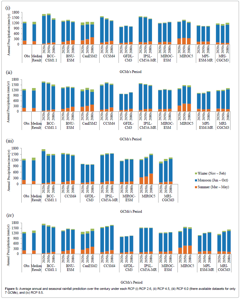
Figure 5: Average annual and seasonal rainfall prediction over the century under each RCP (i) RCP 2.6, (ii) RCP 4.5, (iii) RCP 6.0 (there available datasets for only 7 GCMs), and (iv) RCP 8.5.
With reference to the median of multi-GCMs result, the annual rainfall in the upcoming century is likely to slight increase in most of the scenarios. The BCC-CSM1.1 and CCSM4 models show an increase in annual rainfall in most RCPs scenarios (+37.53% and +32.26% of the observed annual rainfall respectively). In contrast to this, GFDLCM3 and MPI-ESM-MR models show the decrease in rainfall (-20.67% and -14.65% of the observed annual rainfall respectively). The monthly changes under each climate scenario are also shown in Figure 6.
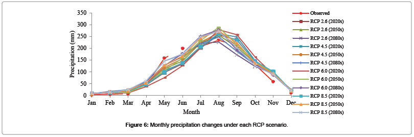
Figure 6: Monthly precipitation changes under each RCP scenario.
An increasing trend in temperature is expected in near future (Figures 7 and 8). Extremes of both maximum and minimum temperature are likely to occur in summer period. Temperatures will reach to the highest records in the 2080s period under RCP 8.5 scenario (maximum and minimum temperatures of 33.19°C and 24.35°C). Maximum temperature will deviate from the baseline values in the range of -0.53°C~4.00°C in summer, 0.26°C ~3.20°C in monsoon and -0.94°C~3.20°C in winter. Similarly, minimum temperature will fluctuate within -1.24°C~8.01°C of baseline in summer, 0.50°C~3.97°C in monsoon and -0.30°C~6.58°C in winter. Both temperature extremes have steepest increasing trends at later period in RCP 8.5. Detail changes under respective climate scenarios are summarized in Table 4a,4b and 4c.
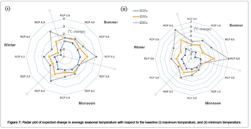
Figure 7: Radar plot of expected change in average seasonal temperature with respect to the baseline (i) maximum temperature, and (ii) minimum temperature.
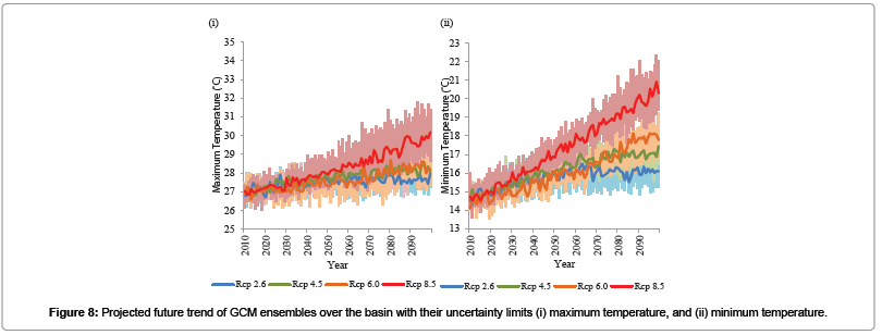
Figure 8: Projected future trend of GCM ensembles over the basin with their uncertainty limits (i) maximum temperature, and (ii) minimum temperature.
Annual resolution: In the early future period (2020s) the average annual rainfall over the whole basin has decreasing trend at Lawpita, Namsang, Pinlaung, Taunggyi, Loilem, and Mobye stations. Out of the mentioned in the first three stations, the decreasing trend is usually found in all RCPs of the early period (2020s). In the middle (2050s) and late (2080s) period rainfall is expected to increase across the basin. Extreme rainfall events are mostly found around Loikaw and Heho stations. The maximum increase in rainfall is found in Heho station, 16.63% and Loikaw station, 19.72% at the late period under RCP 8.5.
Comparing those deviations at the stations, the biggest rise in maximum temperature occurs in Namsang for all the climate scenarios (1.64°C, 2.17°C, 2.17°C and 4.08°C at the end of 21st century under RCP 2.6, 4.5, 6.0 and 8.5 scenarios respectively). Heho and Namsang stations show highest increase in minimum temperature. At Namsang station, the increase in minimum temperature are 2.92°C, 3.81°C, 4.50°C and 6.81°C at the end period of RCP 2.6, 4.5, 6.0 and 8.5 respectively. Loikaw station is the least sensitive to both maximum and minimum temperature changes in all future scenarios.
Referring to Figure 7, out of all four RCP scenarios, the steepest trend is shown by RCP 8.5. On the other hand, RCP 4.5 and 6.0 fluctuate in terms of higher trend. Although RCP 6.0 shows lowest trend in late period it eventually ends up at second highest position in terms of temperature magnitude at the end of the century. The final magnitude attained by RCP 6.0 and 4.5 are distinct from each other for minimum temperature while there is not much difference for maximum temperature. Although both temperature extremes are projected to increase, minimum temperature will face greater change (+1.87°C, +2.78°C, +3.23°C and +5.27°C under later period of RCP 2.6, 4.5, 6.0 and 8.5 respectively) than maximum temperature (+1.13°C, +1.58°C, +1.61°C and +2.82°C under late period of RCP 4.5, 2.6, 6.0 and 8.5 respectively). So, minimum temperature is estimated to undergo almost double the change as compared to the projected changes in maximum temperature.
Spatial variability analysis on future basin water management
The Inle lake area and downstream most portions of the basin are likely to receive more rainfall in future (Figure 9). But, in the middle hilly region between Inle lake and Mobye reservoir a decreasing trend is noticed in RCP 2.6. A slight increase exists in RCP 4.5 and RCP 6.0 compared to RCP 2.6. However, the average rainfall over the basin in RCP 4.5 and RCP 6.0 scenarios is still greater than the observed historical period. Whereas with RCP 8.5, even the middle region is estimated to get an increase in rainfall. These results indicate relative increase in the inflow of water to the Inle Lake. However, the inflow into the Mobye reservoir is affected by both the wet Inle lake area and the drier middle hills. So only a slight increase in inflow at Mobye reservoir is expected under RCP 4.5 and RCP 6.0. However, under RCP 8.5, both Inle lake and Mobye will have higher inflow. There is also relatively increasing trend in Southern portion of basin covering Lawpita hydropower stations. Thus proper control on the releasing water from Mobye reservoir should also be considered to cover the possible flooding of downstream areas (like Loikaw city) due to excess inflow.
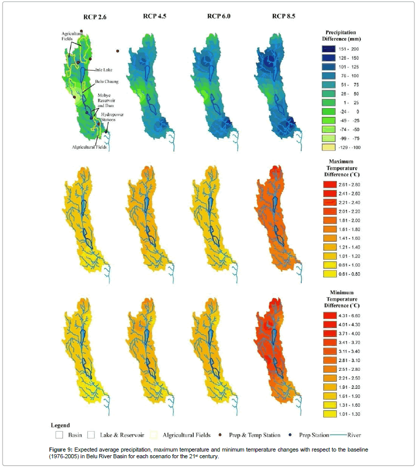
Figure 9: Expected average precipitation, maximum temperature and minimum temperature changes with respect to the baseline (1976-2005) in Belu River Basin for each scenario for the 21st century.
The average maximum temperature over the region has increasing trend for all the climate scenarios in all parts of the region according to Figure 9. But, all the surrounding areas of Inle lake, Mobye reservoir and the middle region of basin have a lower increasing rate comparing to the downstream portion of the basin. Between the two, the evaporation rate at Inle lake is expected to be higher than that of Mobye reservoir. Similarly, the increasing trend in minimum temperature is expected all over the region under all RCPs but at a higher rate. Compared to the middle hills, the change in minimum temperature at Inle lake catchment area and the downstream most portion of the basin are greater. For both temperature extremes there is only slight difference in average increment of temperature between RCP 4.5 and RCP 6.0 scenarios. Due to most likely increase in average temperature and evaporation losses in the reservoir, it is necessary to plan on optimizing water usage for the irrigation area around Loikaw city.
Conclusions
This paper aims to project future climate scenarios of Belu River Basin of Myanmar. Future climate data of ten GCMs were bias corrected by using quantile mapping technique. Projection of precipitation shows mix results across the basin. The basin average values of precipitation suggest both a slight increasing and a slight decreasing trend (-1.78~+9.14%). Distinct drop in rainfall in May (-52.04%~-7.44%) shows the monsoon is going to get delayed. Although the peak rainfall is still found in August as observed rainfall, the higher intensity of increase which is up to -3.36%~+23.23% is noticed in future projection scenarios. In addition, only two (July and August) out of five months of monsoon getting large boost in magnitude for all periods indicates monsoon hydrograph to be narrower and higher intensity with more extreme events.
Both temperature extremes are likely to rise in the coming century. The increasing rate of minimum temperature (+0.64~+5.27°C) is found to be higher than that of maximum temperature (+0.56~+2.82°C) for each period. May is the most affected month (+2.10~+4.00°C) for maximum temperature while March is inflicted the most for minimum temperature (-1.24~+8.01°C).
Analysis of spatial distribution of climate change impact shows downstream/southern part of the basin as most affected. The Inle lake, Mobye dam and their surrounding area will receive increase in rainfall and temperature. Due to the increasing trend of temperature, the Mobye reservoir is expected to lose more water was evaporation. This likely change should be put under consideration in the future operation of hydropower plants. Major cultivation fields are situated in highest temperature increase zone which leads to the possibility of increase in future water requirement from Mobye reservoir. Additionally late monsoon, high intensity rainfall in July and August, and the gradual increase in temperature are also noted as the highly possible climate phenomenon of the study area in coming century. In comparison to the southern portion the northern/ upstream portion is less likely to suffer major changes under climate change scenarios.
The Belu River Basin has a multi-faceted water-energy-food interlinkage. Climate change analysis studies such as this is crucial to policy makers and stakeholders in decision making. There is no doubt, actions taken in timely manner will aid to offset the negative impact of climate change on the existing and future water resource management systems as well as the operation works of hydraulic structures.
Acknowledgement
The authors acknowledge the financial support provided by a Norwegian Scholarship and by the Asian Institute of Technology, Thailand, to conduct this research. The authors would also like to thank the Department of Meteorology and Hydrology, Ministry of Electricity and Irrigation Department of Myanmar for providing important and valuable data for the research.
References
- Nunez M, McGregor JL (2007) Modelling future water environments of Tasmania, Australia.Clim Res 34 25-37.
- Helfer F, Lemckert C, Zhang H (2012) Impacts of climate change on temperature and evaporation from a large reservoir in Australia. Journal of Hydrology 475: 365-378.
- Chen J, Brissette FP,Leconte R (2011) Uncertainty of downscaling method in quantifying the impact of climate change on hydrology. J Hydrol 401: 190-202.
- Johnson F, Sharma A (2011) Accounting for interannual variability: A comparison of options for water resources climate change impact assessments. Water Resour Res 47.
- Teutschbein C, Seibert J (2013) Is bias correction of regional climate model (RCM) simulations possible for non-stationary conditions? Hydrol Earth Syst Sci 17: 5061-5077.
- Kundzewicz ZW, Mata LJ, Arnell NW, Döll P, Jimenez B, et al. (2008) The implications of projected climate change for freshwater resources and their management.Hydrol Sci J 53: 3-10.
- Bosshard T, Carambia M, Geoergen K, Kotlarski S, Krahe P, et al. (2012) Quantifying uncertainty sources in an ensemble of hydrological climate-impact projections. Water Resources Research 49: 1-14.
- Smith I, Chandler E (2010) Refining rainfall projections for the Murray Darling Basin of south-east Australia-the effect of sampling model results based on performance. Climatic Change 102: 377-393.
- Lutz AF,Immerzeel WW,Gobiet A,Pellicciotti F,Bierkens MFP (2013) Comparison of climate change signals in CMIP3 and CMIP5 multi-model ensembles and implications for Central Asian glaciers.Hydrol Earth Syst Sci 17: 3661-3677.
- Kotsiantis S, Kostoulas A, Lykoudis S, Argiriou A,Menagias K (2006) Filling Missing Temperature Values in Weather Data Banks. 2nd IEE International Conference on Intelligent Environmentsin Athens, Greece, USTARTH 1: 327-334.
- Agarwal A, Babel MS,MaskeyS (2014) Analysis of future precipitation in the Koshi river basin Nepal J Hydrol 513: 422-434.
- Yatagai A, Kamiguchi K, Arakawa O, Hamada A, Yasutomi N,et al. (2012) APHRODITE: Constructing a Long-Term Daily Gridded Precipitation Dataset for Asia Based on a Dense Network of Rain Gauges. B Am Meteorol Soc 93: 1401-1415.
- Immerzeel WW, BeekVLPH,Bierkens MFP (2010) Climate change will affect the Asian water towers. Science 328: 1382-1385.
- Hawkins E, Sutton R (2011) The potential to narrow uncertainty in projections of regional precipitation change.ClimDynam 37: 407-418.
- Teutschbein C, Siebert J (2012) Bias correction of regional climate model simulations for hydrological climate-change impact studies: Review and evaluation of different methods. Journal of Hydrology 456-457: 12-29.
- Lafon T, Dadson S, Buys G,Prudhomme C (2013) Bias correction of daily precipitation simulated by a regional climate model: a comparison of methods. International Journal of Climatology 33: 1367-1381.
- Gudmundsson L, Bremnes JB, Haugen JE, Engen-Skaugen T (2012) Thechnical Note: Downscaling RCM precipitation to the station scale using statistical transformations-a comparison of methods.Hydrol Earth Syst Sci 16: 3383-3390.
- Piani C, Haerter JO, Coppola E (2010) Statistical bias correction for daily precipitation in regional climate models over Europe. Theor AplClimatol 99: 187-192.
- R Development Core Team (2011) R: A language and Environment for Statistical Computing, R Foundation for Statistical Computing. Vienna, Austria.
- Gudmundsson L (2015) Package Qmap-Statistical transformations for post-processing climate model output.
- Chaturvedi RK, Joshi J, Jayaraman M, Bala G,Ravindranath NH (2012) Multi-model climate change projections for India under representative concentration pathways. Current Science 103.
- Miao C, Duan Q, Sun Q, Huang Y, Kong D, et al. (2014) Assessment of CMIP5 climate models and projected temperature changes over Northern Eurasia. IOP Publishing Environ Res Lett 9: 12.
- Infrastructure for the European Network for Earth System Modelling (IS-ENSE) Exploring climate model data.
- Intergovernmental Panel on Climate Change (IPCC) (2009)Fifth Assessment Report (AR5).
- NCAR UCAR The Climate Data Guide-APHRODITE: Asian Precipitation-Highly-Resolved Observational Data Integration Towards Evaluation of Water Resources.available at: https://climatedataguide.ucar.edu/climate-data/aphrodite-asian-precipitation-highly-resolved-observational-data-integration-towards.
- https://climatedataguide.ucar.edu/climate-data/aphrodite-asian-precipitation-highly-resolved-observational-data-integration-towards
Citation: Aung MT, Shrestha S, Weesakul S, Shrestha PK (2016) Multi-model Climate Change Projections for Belu River Basin, Myanmar under Representative Concentration Pathways. 7: 323. DOI: 10.4172/2157-7617.1000323
Copyright: © 2016 Aung MT, et al. This is an open-access article distributed under the terms of the Creative Commons Attribution License, which permits unrestricted use, distribution, and reproduction in any medium, provided the original author and source are credited.
Select your language of interest to view the total content in your interested language
Share This Article
Recommended Journals
Open Access Journals
Article Tools
Article Usage
- Total views: 12794
- [From(publication date): 1-2016 - Aug 30, 2025]
- Breakdown by view type
- HTML page views: 11735
- PDF downloads: 1059