Patterns of Total Precipitation for the City of Rio de Janeiro (1961-2013): Evidence of Normality and Inter Seasonal Correlations
Received: 11-Feb-2014 / Accepted Date: 27-Feb-2014 / Published Date: 02-Mar-2014 DOI: 10.4172/2157-7617.1000190
Abstract
Using data from the Praça Mauá meteorological station located on Rio de Janeiro (Latitude: -22.88, Longitude: -43.18, Altitude: 11.10m), twelve histograms and normal probability plots were obtained utilizing all available historical data for each month, between the years of 1961 and 2013. The normality of the distributions was evaluated using the Shapiro-Wilk test. From these results a profile for each month’s and season’s distribution patterns was obtained. This, in turn, may complement the current understanding of the intense rain events approached in other studies using the method of searching for intensity, duration and frequency curves (IDF) for the city of Rio de Janeiro, especially for the cases of urban infrastructure planning associated with hydrological and hydraulic dimensioning studies. Gaussian-like distributions were observed for all seasons separately, and for the months of May, October, November and December individually. Spearman and Pearson tests showed positive correlations, in some cases, between total precipitations for each season throughout the historical series.
Keywords: Total precipitation; Historical average; Normality
5897Introduction
Precipitation and natural disasters in Brazil
According to the Emergency Disasters Database [1], floods are one of the major recurrent types of natural disasters in Brazil throughout the years of 1900 to 2013, and comprise the bottom half of the ten natural disasters that affected most people, as well as six out of the top ten disasters sorted by numbers of killed and by economic damage costs.
The city of Rio de Janeiro is often affected by such types of situations. A natural disaster occurs whenever natural phenomena of great intensity have impact over an area, or a populated region, and may or may not be aggravated by anthropic activities [2]. Recent examples include two disasters in the years of 2010 and 2011. On the first, on the beginning of April 2010, daily precipitation accumulations of more than 150 mm were recorded in several zones of the Metropolitan Region of Rio de Janeiro. On the second, 222 mm of precipitation were measured in just twelve hours.
Both events caused floods and earth slides, resulting in massive damage, especially in areas with less urban planning and more precarious infrastructure. This can be even more problematic since rain tends to fall 5 to 10% more in medium and large cities, when compared to rural areas [3]. This difference may be attributed to effects caused by urban heat islands that generate convection, by the rugosity associated with the numerous edifications that cause turbulence and by the amount of pollution particulate material suspended in air that increases the propensity of cloud formation by acting as hygroscopic nuclei.
Since natural disasters have been shown to correlate with the occurrence of massive rainfalls, it becomes imperative to better grasp the origins of such precipitation accumulations, or to identify whichever patterns that might lead to a more complete understanding of them. Several studies have been performed on the subject, trying to pinpoint causes with different approaches, many of which have been summarized by Moura [4].
Some of these studies try to find correlations between total precipitation amounts and other factors such as the propensity of earth slides or other types of disasters. Episodes with total recorded precipitations at least 20% higher than the yearly average tend to develop catastrophic proportions [5].
Intense rainfall studies
Some lines of studies regarding intense rainfall events approach the subject with the search for intensity, duration and frequency equations. These are basically equations that allow for predictions of precipitation levels based on the duration of the event, the return time, the location and the physiographical characteristics of the region. These equations might arise in different forms depending on how they are derived from the ones found by Pfafstetter [6] or which parameters are being focused on.
The city hall of Rio de Janeiro has, in at least two studies, suggested the usage of IDF equations for hydric planning and predictions of flow measurements for drainage constructions [7,8]. In both studies the IDF equations are cited as the tool that should be preferred for prediction of intensities on the more severe rainfall events, and are key for elaborating projects of drainage systems to avoid floods. These equations depend on several parameters, one of which is the mean yearly precipitation [9].
However, this quantity does not reflect, by itself, the intricacies and differences in the general larger behaviour of precipitation distributions on each month of the year. While it is not trivial to assume if this hinders or not the efficacy of the IDF equations, or if they could be further enhanced by using a parameter more sensitive to each month’s contribution (the simplest example being a weighted mean with fitted weight parameters), it becomes compelling to attempt to better understand the monthly precipitation distribution’s profiles and properties.
This study aims to provide a description of such patterns using statistical analyses of historical total precipitation data, for each month individually and also grouping them by season. Another result attained is the pattern of precipitations above the historical averages for each month, using data from approximately thirty years of measurements. This might help to understand on which months it should be more expected, or rather less than a surprise, for the historical average to be surpassed more often, and possibly have applications in climate impact or water supply related research. These results are something that the simple usage historical averages as first guesses would not provide.
Materials and Methods
Data choice
Monthly total precipitation measurements were obtained from the BDMEP database, which is provided by the Instituto Nacional de Meteorologia (INMET). The closest station available on the system with monthly measurements is the Praça Mauá meteorological station, with latitude: -22.88, longitude: -43.18 and altitude: 11.10m. Figure 1 shows the localization of this station.
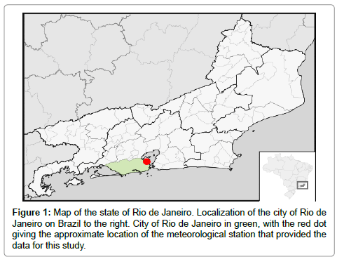
Figure 1: Map of the state of Rio de Janeiro. Localization of the city of Rio de Janeiro on Brazil to the right. City of Rio de Janeiro in green, with the red dot giving the approximate location of the meteorological station that provided the data for this study.
For the months from January to April, there was available data from 1961 to 1983 and then from 2003 to 2013, totalizing 34 years of data. Similarly, from May to September, the available data was from 1961 to 1983 and then from 2002 to 2013, adding up to 35 years of data. Lastly, from October to December, the database had measurements from 1961 to 1983 and then from 2002 to 2012, totalizing 34 years of measurements as well. To allow for comparison, as well as correlation studies, only years where all months are available where used, i.e. 1961 to 1983 and 2002 to 2012, resulting in a population size of 33.
To gather information about the different seasons, starting from the original set of monthly data, an approximation had to be made.
Since the seasons generally start around the twentieth day of the month, roughly two thirds of the last month of a season corresponds to the season that is ending at that point, and one third corresponds to the season beginning.
The approximation made can is explained in the following example: To calculate the total precipitation of the fall season of a specific year, the sum of one third of the precipitation of March of that year, the entire precipitations of April and May, and two thirds of the precipitation of June was computed, as approximately two thirds of March correspond to the summer, while one third corresponds to fall.
This approximation provided a rough, qualitative idea of the patterns, which could however still be invaluable for the reasons previously stated.
There is another important detail, regarding the calculations for summer, since this season always starts on a particular year and ends on the following one. To compute the total precipitation for this season for a given year, the data used was one third of December’s total, for that year, and then the total precipitations from January, February and two thirds from March, from the year following. For this reason the summer of 2013 could not be evaluated, and the year of 2013 was suppressed from the seasonal analysis resulting in a sample size of 32.
Statistical analysis
Separating data by month, twelve histograms and Quantile-quantile plots (Q-Q Plots) were generated. The distributions and patterns on these were tested for normality using Shapiro-Wilk tests because these have been shown to outperform other common normality tests, especially for asymmetric distributions of population sizes of about 30 [10]. However, since the power of such normality tests is lower for smaller sample sizes, these results are to be taken as qualitative rough first estimates, and have been complemented by a graphical analysis by inspection of the histograms and Q-Q Plots. After this, data was grouped by season, and four more histograms where obtained and the distributions tested by a similar approach.
It was also desirable to check for possible correlations of the measured data between seasons and with the passage of years, with both Pearson and Spearman tests being used. Taking into account that the former is better suited to find linear correlations between normal variables, while the latter does so for distributions that are neither necessarily parametric nor linearly correlated; both tests were used, because even with the normal behaviour of the seasonal distributions calculated at a later point, one could not assume correlations being linear beforehand.
Lastly a few attempts of fitting convoluted distributions to some sets of data were attempted to further try to reveal patterns using CERN’s ROOT data analysis framework. All other statistical data was analysed using IBM’s SPSS Statistics 20.
Results and Discussion
Table 1 shows the results for the normality tests. The Shapiro- Wilk test determined that May, October, November and December are the months that correspond the most to normal distributions, with November being the month that most approached it. For these months, then, one could use basic statistics to predict that most total precipitations should fall within a few standard deviations from the historical mean, with the possibility of choosing how rigid the predictions would be by increasing the number of standard deviations. A typical three standard deviation approach (representing 99.73% of the distribution) would be enough to account for potentially disastrous rains where a rough estimate using the mean value wouldn’t. Choosing this upper value could be of use for infrastructural planning, and the number of standard deviations chosen would be limited by cost or logistic factors.
| Shapiro-Wilk | |||
|---|---|---|---|
| Statistic | df | Sig. | |
| January | .915 | 33 | .013 |
| February | .872 | 33 | .001 |
| March | .888 | 33 | .003 |
| April | .877 | 33 | .001 |
| May | .963 | 33 | .312 |
| June | .869 | 33 | .001 |
| July | .891 | 33 | .003 |
| August | .862 | 33 | .001 |
| September | .859 | 33 | .001 |
| October | .962 | 33 | .286 |
| November | .979 | 33 | .757 |
| December | .963 | 33 | .311 |
Table 1: Tests of Normality
To corroborate this result, the histograms shown in Figure 2 have both the means and standard deviations displayed as well as the Gaussian curve corresponding to these quantities plotted over the data for a graphical analysis, and Q-Q plots are shown in Figure 3. The overall aspect of the distribution matches the normality tests results.
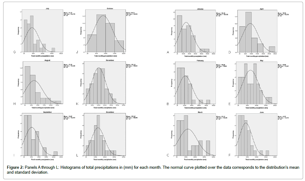
Figure 2: Panels A through L: Histograms of total precipitations in (mm) for each month. The normal curve plotted over the data corresponds to the distribution's mean and standard deviation.
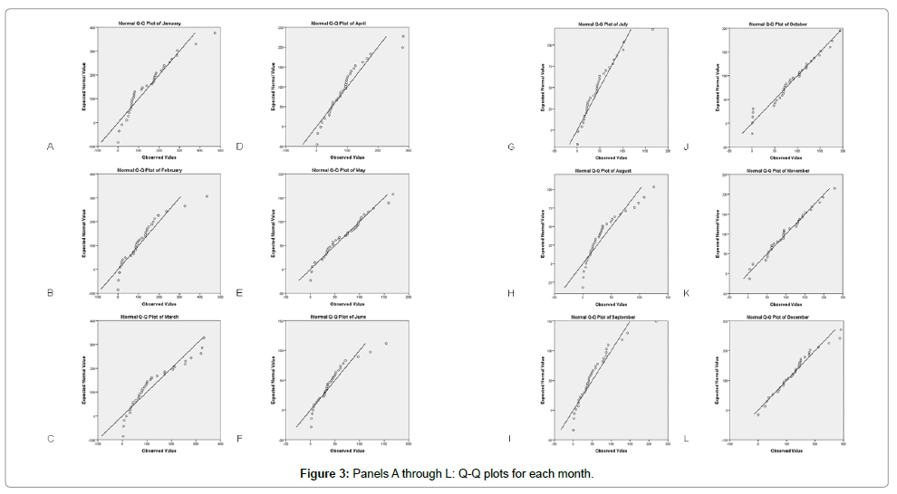
Figure 3: Panels A through L: Q-Q plots for each month.
In all months a sometimes slight, sometimes more pronounced asymmetry in favour of small precipitation values was observed. This suggested that rough modelling or curve fitting attempts regarding this data, even for the months with Gaussian-like distributions, would be improved by usage or convolution with asymmetrical, positively skewed distributions, such as log-normal, logarithmic, landau or other such distributions, or even possibly a decaying exponential one.
One such example of this is shown in Figure 4 where the data from the December histogram was fitted twice using different approaches. The first was to let ROOT fit the best Gaussian it could find, and see what outputs it gave in terms of its probability function, which is based on the chi-squared calculated values and gives a rough idea of how well the fitting process performed (a probability of 1 being a perfect fit). Then another fitting attempt was made, this time using a trial function that was a convolution of a Gaussian and a decaying exponential distribution. Although graphical analysis shows that the fitting is not perfect, this already shows improvement, which is also seen in the increase of the probability value. However, since one is more interested in the higher values of precipitation, for these are usually correlated to the natural disasters in Rio de Janeiro, a qualitative understanding of the distribution’s patterns should be sufficient for rough estimates.
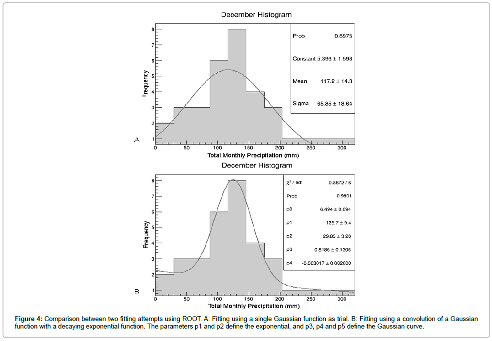
Figure 4: Comparison between two fitting attempts using ROOT. A: Fitting using a single Gaussian function as trial. B: Fitting using a convolution of a Gaussian function with a decaying exponential function. The parameters p1 and p2 define the exponential, and p3, p4 and p5 define the Gaussian curve.
For the months with distributions farther from normal, one can qualitatively see from the histograms that a recurring pattern is that the deviations from normality occur more strongly for lower precipitation values as a general rule, suggesting that one would still use the three standard deviations approach for upper limit estimations, except for March, where frequency of higher valued precipitations increase sharply around the 300 to 350 mm range. Possibly a more rigid criteria could be chosen for this month, for these reasons.
The seasonal histograms, as well as normality tests applied to these distributions, reveal that the contributions of the months add up to roughly normal distributions for all seasons as shown in Figures 5 and 6 and Table 2. This could be important information regarding rough estimates of average seasonal or even yearly precipitations, and it gives a sounder base for a three standard deviation approach as described previously.
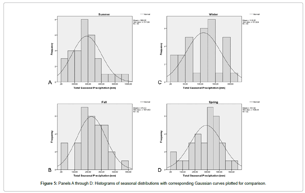
Figure 5: Panels A through D: Histograms of seasonal distributions with corresponding Gaussian curves plotted for comparison.

Figure 6: Panels A through D: Q-Q plots of seasonal distributions.
| Shapiro-Wilk | |||
|---|---|---|---|
| Statistic | df | Sig. | |
| Fall | .979 | 32 | .776 |
| Winter | .965 | 32 | .382 |
| Spring | .964 | 32 | .342 |
| Summer | .951 | 32 | .150 |
Table 2: Tests of Normality.
Table 3 shows the results for the Pearson and Spearman correlation tests. There was no clear immediate correlation indicated by these tests for this period regarding either increase or decrease of seasonal total precipitations with the passage of time, except for the spring season, which presented a positive Pearson correlation. However, positive correlations, some of which with significance at 0.01 level, were shown between seasons. Summer and winter correlate to their immediately adjacent seasons; fall correlates to winter and spring, and spring seems to correlate with all the others. This could represent another possible criterion for rough estimation of average behaviour for seasons, especially on the case of summer, which is where most disasters happen. Years with high levels of precipitation for spring would suggest extra care regarding summer.
| Year | Fall | Winter | Spring | Summer | |||
|---|---|---|---|---|---|---|---|
| Spearman | Fall | Correlation Coefficient | 0.083 | 1 | ,409* | 0.323 | 0.216 |
| Sig. (2-tailed) | 0.652 | 0.02 | 0.071 | 0.234 | |||
| N | 32 | 32 | 32 | 32 | 32 | ||
| Winter | Correlation Coefficient | 0.034 | ,409* | 1 | ,538** | 0.335 | |
| Sig. (2-tailed) | 0.855 | 0.02 | 0.001 | 0.061 | |||
| N | 32 | 32 | 32 | 32 | 32 | ||
| Spring | Correlation Coefficient | 0.26 | 0.323 | ,538** | 1 | ,382* | |
| Sig. (2-tailed) | 0.151 | 0.071 | 0.001 | 0.031 | |||
| N | 32 | 32 | 32 | 32 | 32 | ||
| Summer | Correlation Coefficient | -0.207 | 0.216 | 0.335 | ,382* | 1 | |
| Sig. (2-tailed) | 0.255 | 0.234 | 0.061 | 0.031 | |||
| N | 32 | 32 | 32 | 32 | 32 | ||
| Year | Fall | Winter | Spring | Summer | |||
| Pearson | Fall | Correlation Coefficient | 0.173 | 1 | ,522** | ,513** | 0.296 |
| Sig. (2-tailed) | 0.343 | 0.002 | 0.003 | 0.1 | |||
| N | 32 | 32 | 32 | 32 | 32 | ||
| Winter | Correlation Coefficient | 0.116 | ,522** | 1 | ,599** | 0.265 | |
| Sig. (2-tailed) | 0.527 | 0.002 | 0.00029 | 0.143 | |||
| N | 32 | 32 | 32 | 32 | 32 | ||
| Spring | Correlation Coefficient | 0.382 | ,513** | ,599** | 1 | 0.418 | |
| Sig. (2-tailed) | 0.031 | 0.003 | 0.00029 | 0.017 | |||
| N | 32 | 32 | 32 | 32 | 32 | ||
| Summer | Correlation Coefficient | -0.129 | 0.296 | 0.265 | 0.418 | 1 | |
| Sig. (2-tailed) | 0.482 | 0.1 | 0.143 | 0.017 | |||
| N | 32 | 32 | 32 | 32 | 32 | ||
*Correlation is significant at the 0.05 level (2-tailed).
Table 3: Correlations.
Conclusion
Thirty-three years of data taken from monthly precipitations in Rio de Janeiro were investigated for normality and correlation. Normality was observed in May, October, November and December, and also for all cases when the months were grouped by season, with May are being the most Gaussian-like monthly distribution and fall’s the most seasonal one. This suggests using an upper limit estimated as a certain number of standard deviations above historical mean as a representative value for a rough description of the precipitation distributions.
For months with non-Gaussian distributions the deviations from normality seem to occur in greater part due to lower valued total precipitations. This also indicates that similar approaches of choosing upper limits defined by a number of standard deviations over the mean value rather than mean value itself could be useful when surveying for yearly averages to further complement or aid whichever projects or techniques that rely on that particular information, or simply to have an qualitative estimate or a rough first guess. These results could perhaps aid in understanding of intense rain patterns and complement actions taken to avoid potential natural disasters.
Since the statistical approach used is rather simple, it could prove to be an invaluable, readily feasible form of studying patterns of intense rainfalls in locations where more complex studies involving other techniques cannot be performed, as well as give more information for urban infrastructure and planning on those areas, regarding flood management.
Acknowledgement
The authors acknowledge the Instituto Nacional de Meteorologia (Inmet) for providing the data used in this study.
References
- EM-DAT (2013)The OFDA/CRED International Disaster Database.Universitécatholique de Louvain – Brussels-Belgium.
- Castro ALC (1999) Manual de planejamento em defesa civil. Ministério da Integração Nacional/Departamento de Defesa Civil,BrasÃlia.
- Moura CRW, Escobar GCJ, Andrade KM (2013) Padrões de circulação em superfÃcie e altitude associados a eventos de chuva intensa na região metropolitana do rio de janeiro.Rev Brasileira de Meteorologia 28: 267-280.
- Guidicini G, Iwasa OY (1976) Ensaio de correlação entre pluviosidade e escorregamentos em meio tropical úmido. Instituto de Pesquisas Tecnológicas do Estado de São Paulo SA: 48.
- Pfafstetter O (1982) Chuvas Intensas no Brasil, Rio de Janeiro, DNOS, Planer/Fundenor. Estudos Hidrológicos/Determinação de vazões para obtenção de outorga de água nas bacias hidrográficas de interesse do Programa Moeda Verde Rio Cana: 426.
- Instruções técnicas para elaboração de estudos hidrológicos e de dimensionamento hidráulico de sistemas de drenagem urbana (2013) Secretaria Municipal de Obras; Subsecretaria de Gerenciamento de BaÃas Hidrográficas-Rio águas.
- Plano estadual de recursos HÃdricos do Estado do Rio de Janeiro (2013) Secretaria de Estado do Ambiente; Instituto Estadual do Ambiente.
- Davis EG, Naghettini MC (2001) Estudo de Chuvas Intensas no Estado do Rio de Janeiro. Companhia de Pesquisa de Recursos Minerais, Brasil.
- Razali NM, Wah YB (2011) Power comparisons of Shapiro-Wilk, Kolmogorov-Smirnov, Lilliefors and Anderson-Darling tests. J Statistical Mod el Anal 2: 21-33.
Citation: Palatnik de Sousa I, Palatnik de Sousa CB (2014) Patterns of Total Precipitation for the City of Rio de Janeiro (1961-2013): Evidence of Normality and Inter Seasonal Correlations. J Earth Sci Clim Change 5: 190. DOI: 10.4172/2157-7617.1000190
Copyright: ©2014 Palatnik de Sousa I, et al. This is an open-access article distributed under the terms of the Creative Commons Attribution License, which permits unrestricted use, distribution, and reproduction in any medium, provided the original author and source are credited.
Select your language of interest to view the total content in your interested language
Share This Article
Recommended Journals
Open Access Journals
Article Tools
Article Usage
- Total views: 15235
- [From(publication date): 4-2014 - Sep 02, 2025]
- Breakdown by view type
- HTML page views: 10572
- PDF downloads: 4663