Journal of Earth Science & Climatic Change
Open Access

The fifth IPCC Assessment Report (IPCC,2014) confirms the increase in the Earth's average temperature and that this rapid change in the global climate may result in an increase of the frequency and intensity of extreme events and natural disasters (cyclones and storms, heat waves and droughts, heavy precipitation and floods, etc.) by the end of the 21st century. The Mediterranean basin is one of the most vulnerable regions with respect to global warming, notably because 43 of strong air-sea interactions [1]. In this area, the complexity of the basin topography with a semi closed sea-located between a semiarid to arid region in the south and a temperate climate in the northsurrounded by a high coastal orography, calls for the consideration of the different components of the Earth system when studying intense events.

Heavy Precipitation Events (HPEs) are characterized by daily amounts of precipitation larger than 100 mm occur frequently in the Northwestern MEDiterranean (NWMED) [2]. The Cévennes-Vivarais (CV) region (Figure 1) in the southeast of France particularly suffers from HPEs. Those HPEs and the floods often associated might cause ecological effects, large economic damage and human casualties. The remarkable event of 8-9 September 2002 [3] with nearly 700 mm recorded in 24 h over the Gard region resulted in 20 deaths and estimated to be of more than one billion Euros [4]. With a cluster analysis [5] we investigate the atmospheric synoptic circulation over the north Atlantic and Western Europe related to HPEs in different regions of the NWMED, considering the different stages of an HPE: initiation, maturity and dissipation. The CV region has been found to be related mostly to a strong Cyclonic South Westerly (CSW) flow. During the mature stage of the HPE, the CSW cluster is characterized by the following features: a deep 500hPa trough from northwest of the British Islands extending southwards to the Bay of Biscay, a deep lowpressure system above the Channel and southwesterly winds above Western Europe at sea level. The CSW is related to the appearance of a low-level jet which transports the heat and moisture extracted from sea. As the low-level air mass reaches the Massif Central relief, it reaches its maximum potential energy. With addition to an uplift effect in the Gulf of Lions (GOL; that will be described later on), it results in convection and precipitation.

A large amount of precipitation could have occurred in association with the cold front over the NWMED, with its slow progression caused by the inland topography (Alps, Massif Central and Pyrenees). However, HPEs are more frequently induced by quasi73 stationary meso-scale convective systems (MCSs). The lifting mechanisms leading to a quasi-stationary MCSs generating the large rainfall amount include orographic lifting, low-level wind convergence and cold pools due to precipitation evaporation [2]. The velocity and the moisture content of the marine low-level flow have been shown to have a significant role on the intensity and location of HPEs [5,6]. The Sea Surface Temperature (SST) largely controls the exchanges between the ocean and the atmosphere, together with the wind patterns which modulate the efficiency of the exchanges. Different studies have shown the influence of SST in the NWMED, on HPEs occurrence, rainfall intensity and spatial distribution of precipitation [7- 9]. They highlight that high SST induces strong air-sea heat fluxes, which moisten and destabilize the atmospheric boundary layer. Focusing on the case studies in the CV region, Lebeaupin Brossier et al. highlight that the low-level jet induces moderate to strong air-sea exchanges (wind stress, heat fluxes and evaporation) which extract heat and moisture from the GOL and also rapidly affect the ocean mixed layer. A significant correlation between precipitation and SST anomalies in the western Mediterranean during the autumn season was notably found by Berthou et al. [10]. They explained the anomalies in SST occurrence with the preceding strong winds coming from a northerly direction (Mistral and Tramontane). Further research, by Lebeaupin-Brossier et al. [11] confirms those cold SST anomalies are caused by the Mistral and Tramontane and demonstrate how the cold SST anomalies are then maintained by the ocean circulation. The cold anomaly strongly decreases the evaporation and limits the moisture extraction from the sea for the following HPE.

This highlights the key role of the general ocean circulation in the GOL for HPEs in which air-sea interactions are significant. The general circulation of the Mediterranean Sea is driven by the cyclonic path of the Atlantic Water entering by the Strait of Gibraltar. Along its path, the Atlantic Water is progressively transformed due to different processes mainly dominated by evaporation that result in denser water that sinks and eventually flows out [12]. In the GOL a cyclonic circulation with a scale of 100 km is present, with a low in the sea surface height and a doming structure in density [13]. Two seasonal modes affect the GOL: a stratified water column between May and November and a mixed column between December and April [14].

The NWMED area is one of the rare places prone to convection and dense-water formation during the winter. The GOL circulation, shown in Figure 1, can be characterized by three main sea features [12]:

The Cyclonic Cell (CC)

The unique topography 116 at the sea bottom forms, traps and enhances the cyclonic circulation [15,16]. The local cyclonic gyre results in a barotropic structure that tends to isolate the weakly stratified water in the area. This area is the main dense water formation region in the western Mediterranean. The occurrence of strong Mistral and Tramontane events (meaning large evaporation and heat loss) during winter can trigger intense mixing of the sea surface layer with the intermediate to deepest layers [17]. It is important to mention that Mistral and Tramontane occur all year long, but the ocean mixing occurs only in winter (in February or March) when the surface water is cooled enough to become unstable [18]. Significant evolutions of SST and Sea Surface Salinity (SSS) occur during autumn in the CC, as the preconditioning phase of the convection is characterized by the mixing of the surface water with the warm and salty Levantine intermediate water underneath it [19].

The Northern Current (NC)

Flows westward then southward during the year, along the continental slope south of the French coasts. Most of the time, the surface current is wide (approximately 40 km) and shallow, except from late January until mid- March, when it becomes narrower, deeper and tends to flow closer to the slope. The transport of water by the NC varies between summer (~1Sv) and winter (~1.5-2Sv) [20,21]. The gyres of the NC vary as well, causing changes in the NC general structure (Marmain, et al., 2014).

The Balearic Front (BF)

The Balearic region is a transition region between the northern part of the GOL and the warm and marked mesoscale eddies coming from the Algerian current. Lopez Garcia et al. [22] showed that the BF has a stable salinity front at the surface, while the thermal gradient varies 140 seasonally. Thus, the salinity gradient is considered the signature of the front? The water transport varies between summer and winter, depending on the Balearic current intensity (summer: ~0.6 Sv, winter: 143 ~0.3 Sv) [21,23] and the Algerian eddies (~0.86 144 Sv) [22]. The aim of this study is to better define SST spatial structures linked to the circulation in the GOL and their temporal variability in relation to HPEs in the CV region induced by a characteristic CSW synoptic situation. For that purpose, the MEDRYS ocean reanalysis at a 1/12˚ resolution [18] was used over the 2000-2011 period to identify the oceanic feature locations and for the calculation of an SST index. Then, a two-step unsupervised cluster analysis method was applied to determine the most typical periods. Finally, the Local Moran's I (LMI) spatial statistical method was used to highlight the areas of significant temporal variability of SST, considering the periods defined with the clustering method. For each considered period, the LMI values reduced to the dates of HPEs initial stage and compared to the average LMI values in order to well characterize the SST variability related to HPEs. The paper is organized as follows. Section 2 presents the data used to identify HPEs in the CV and to evaluate the SST in the GOL. Section 3 details the applied methodology. Section 4 presents and discusses the results obtained. At section 5 conclusions are presented.

HPE selection

The observed precipitation dataset was obtained by using the measurements of 464 rain-gauges in the CV region (Figure 1) collected in the framework of the HyMex (Hydrological cycle in the Mediterranean Experiment) program [6,24] for the 2000-2011 period, only considering the autumn season (±1 month): August to December. An HPE was defined by a threshold of 100 mm per day according to a value given in [2,6] in at least two rain gauges, in order to exclude very local events (Figure 2). shows the number and the monthly distribution obtained for HPEs in the CV region between 2000 and 2011. The majority of HPEs occur during October (33 events) and November (30 events). September and December have equal number of HPEs (17 events) and HPEs occur rarely in August. In order to define the initial stage of each HPE, the hourly precipitation data is examined. The beginning of the initial stage is set when an hourly rainfall amount of more than 10 mm is collected in the preceding 24 hours of the HPE. This is used thento extract the NWMED SST corresponding to each HPE (see section 2.2). In order to distinguish and isolate HPE concerning the CV region which includes a southerly low-level flow over the western Mediterranean Sea, we aim to select only synoptic situations corresponding to the CSW pattern, highlighted in [25] (Figure 3). For that purpose, the geopotential height at 500 hPa pressure level was examined in the NCEP/NCAR reanalysis [26] for each HPE. An index was thus defined to identify a CSW synoptic situation. The following conditions have to be fulfilled:

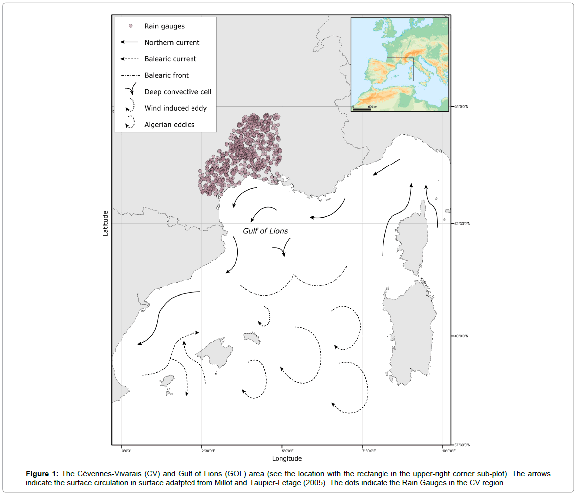
Figure 1: The Cévennes-Vivarais (CV) and Gulf of Lions (GOL) area (see the location with the rectangle in the upper-right corner sub-plot). The arrows indicate the surface circulation in surface adatpted from Millot and Taupier-Letage (2005). The dots indicate the Rain Gauges in the CV region.

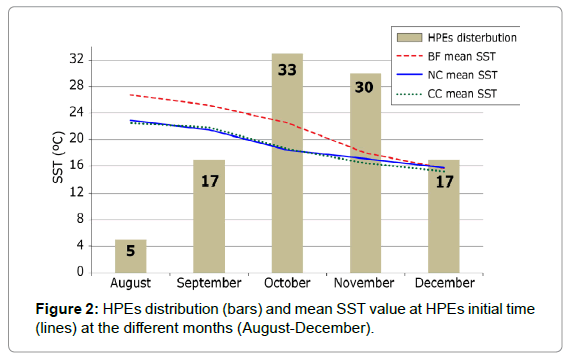
Figure 2: HPEs distribution (bars) and mean SST value at HPEs initial time (lines) at the different months (August-December).

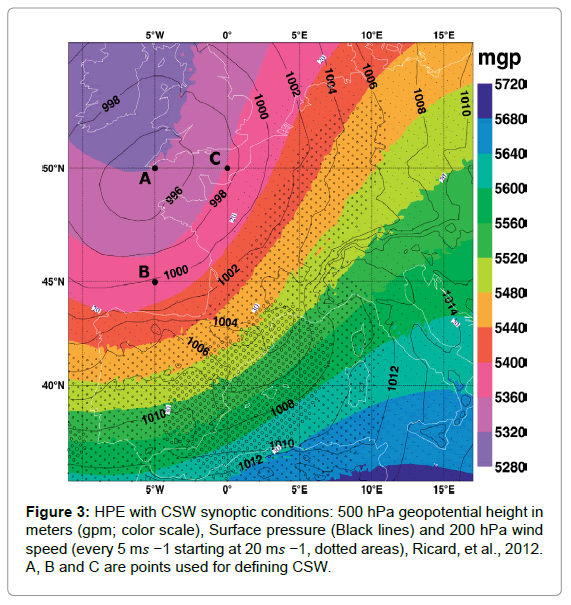
Figure 3: HPE with CSW synoptic conditions: 500 hPa geopotential height in meters (gpm; color scale), Surface pressure (Black lines) and 200 hPa wind speed (every 5 m𝑠 −1 starting at 20 m𝑠 −1, dotted areas), Ricard, et al., 2012. A, B and C are points used for defining CSW.

mgp (A) < mgp (B) (1)

(mgp (B)-mgp (A)) > ( (mgp (C)-mgp (A) (2)

Where mgp is the geopotential height (in meters) and A, B and C correspond to the locations shown in Figure 3. Using this index, we insure that only dates of HPEs that occur during a CSW synoptic condition are selected, thus, we can assume similar heat and moisture sources. It is important to remember that these HPEs occured only during a CSW, while during these months, HPEs with different synoptic patterns might occur.

The Medrys Ocean Reanalysis and the SST Index

The latest version of the MEDiterranean ReanalYsiS [18] MEDRYS1V2 is used. The ocean model used for the MEDRYS reanalysis is NEMO203 MED12 [27], which is the Mediterranean Sea configuration of the NEMO ocean model [28] with a 1/12° (∼7 km) horizontal resolution and 75 vertical z-levels. The atmospheric forcing is ALDERA [18], which is the dynamical downscaling of the ERA- interim atmospheric reanalysis implemented with the regional climate model named ALADIN-Climate. MEDRYS uses the Mercator Ocean data assimilation system SAM2, which is based on a reducedorder Kalman filter, with a three-dimensional (3D) multivariate model decomposition of the forecast error. Altimeter data, satellite SST, and temperature and salinity vertical profiles are jointly assimilated [29]. In the following only the sea surface fields of MEDRYS1V2 will be used. Only the SST field of MEDRYS1V2 over the NWMED area was validated with respect to the Reynolds SST dataset with a 0.25˚ horizontal resolution [30]. Although part of the Reynolds' dataset has been assimilated in MEDRYS1V2, it has been carried out using only one value every 1° in latitude and longitude (to satisfy a noncorrelated dataset hypothesis for the assimilation system), giving one point every 144 NEMO-MED12 grid points; we thus consider the dataset as almost, if not completely, independent. On average over the period 1993-2012, MEDRYS1V2 SST in the NWMED area shows a very small negative bias of -0.07°C: 18.21°C for Reynolds and 18.14°C for MEDRYS1V2 (Figure 4a). Moreover, the monthly cycle is very well represented, with a slight positive bias in winter (JFM), up to +0.07°C in February and a negative bias in spring (AMJ) and summer (JAS), down to -0.22° in May. For the autumn season (OND), the negative bias is small during October - 0.07°C, and smaller during November (-0.03°) and December (-0.02°) as can be seen in Figure 4b. In order to obtain relevant SST indexes, 230 first, the coordinates best describing the three characteristic oceanic features in the GOL, i.e., the Cyclonic Cell (CC), the Northern Current (NC) and the Balearic Front (BF), had to be determined. According to Alberola et al., and Pascual and Gomis [20, 21] the NC coordinates were determined near the coast, at the point 42°47'17''N, 5°40'34''E where it is present during the whole year. The CC location was chosen to be the LION buoy. The coordinates of the closest MEDRYS grid point are 42°0'47''N, 4°41'28''E. The BF was determined using the SSS data. As discussed above, the SSS should more accurately locate the front. In order to have a reference field, a monthly averaged SSS for the total period covered by MEDRYS during 1992-2013 was calculated. Then, a meridional gradient was calculated in the Balearic Islands area (2˚E-4.44˚E, 39.5˚N- 40.73˚N). The maximum value location was defined as the location of the front.

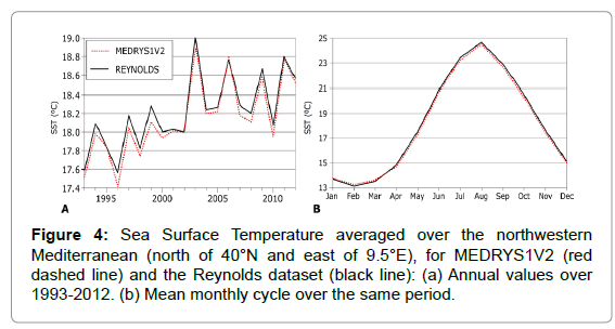
Figure 4: Sea Surface Temperature averaged over the northwestern Mediterranean (north of 40°N and east of 9.5°E), for MEDRYS1V2 (red dashed line) and the Reynolds dataset (black line): (a) Annual values over 1993-2012. (b) Mean monthly cycle over the same period.

(3)

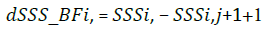
(lon_BF,lat_BF) = lon (MAX (dSSS_BF)), lat (MAX (dSSS_BF) (4)

SSS stands for a SSS monthly average value, and i and j are the rows and the columns respectively. Lon BF and lat_BF stands for the coordinates of the maximum gradient. Please note that only the BF coordinates may vary temporally (Figure 2) shows the SST monthlymean values (of the years 1993-2012) in NC, CC and BF locations. First of all, the gradual (seasonal) decrease in SST is observed from August to December for all the oceanic patterns, except a very small increase in SST in CC between August and September. An interesting point is the relations between each oceanic feature in the different months. August and September seem to have the same relations between the oceanic features (BF>CC≈NC). The October values have the same relations, with lower SST values. November and December were slightly different from other months as the SST values are 254 lower and the gradient between the different oceanic features is very low (BF≈CC≈NC). Then, an SST index (INDSST) merging information on the SST values and pattern using the three ocean-features coordinates was calculated. For that, we choose to weight the SST by the horizontal transport in Sverdrups (Sv) of each feature.

(5)

Because CC is more related to winter months and to vertical transport, the weight (Wcc) was put to zero, thus excluded from that equation. The values for the months of interest (August-December), as described before, are: NC: ∼1.4-1.6 Sv [20,21] BF (made of an average value of the Balearic Current): ∼0.3-0.5 Sv [21,23] and Algerian Eddies: ∼0.86 Sv (Lopez-Garcia etal., 1994) and CC: ∼1-1.2 Sv (Madec et al., 1991). The NC value presented by calculating the average value of 1.4 Sv and 1.6 Sv, resulting in 1.5 Sv. The BF value is a result of averaging 0.4 Sv, representing the Balearic Current contribution, with 0.86 Sv representing the Algerian Eddies. This result in 0.63 Sv. The SST index is calculated only for dates corresponding to HPE initial stages.

(6)

In addition, for the same three points and for the same date, we extracted the 10m-air temperature (Ta) from ALDERA (Ta values above the BF were averaged). This allows calculation of the air-sea thermal gradient (Ta-SST) and thus a relative estimate of the airsea flux intensity (Figure 5) presents a first attempt of HPEs 277 categorization, as a function of the SST index, the air-sea thermal gradient and the months. The radius represents the rainfall amount. The large dependency of the SST index on the month considered is clearly seen. However, no link can be identified with HPEs intensity and/or air-sea thermal gradient. This calls for a further investigation using unsupervised cluster analysis.

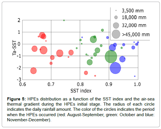
Figure 5: HPEs distribution as a function of the SST index and the air-sea thermal gradient during the HPEs initial stage. The radius of each circle indicates the daily rainfall amount. The color of the circles indicates the period when the HPEs occurred (red: August-September, green: October and blue: November-December).

Clustering method

In order to define temporal clusters, Principle Component Analysis (PCA) was used on the MEDRYS GOL data (2.5˚E-8˚E, 41˚N-43.8˚N). The analysis was held for HPEs initial dates (D) and six consecutive dates prior to it (D-1, D-2, D-3, D-4, D-5, D-6). The PCA is a useful method that allows locating areas of interest. By using eigen value decomposition, the data is projected to a lower dimensional space in the eigen space. This reduction to a 2-D scheme, allows an unsupervised clustering method.

The first PCA calculation was done with Ta-SST matrices (Figure 6a). The correlation of the first component of the PCA (PC1) is 0.47, and the second (PC2) is 0.10, which indicates the amount of data loss due to the dimension-reduction process, are relatively low in this example.

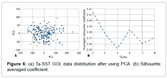
Figure 6: (a) Ta-SST GOL data distribution after using PCA. (b) Silhouette averaged coefficient.

In order to gain better understanding and verification, 301 the same process was implemented solely on SST data (Figure 7a). PC1 is very high (0.88), which means a high correlation between PC1 and SST. The difference between SST analysis and Ta- SST analysis-explained variations stems from the fact that the air temperature varies much more quickly than SST (Figure 7a). PCA data distribution for SST, (b) Averaged Silhouette coefficient value.

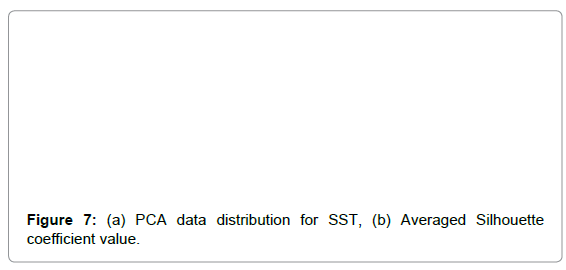
Figure 7: (a) PCA data distribution for SST, (b) Averaged Silhouette coefficient value.

Afterward, the Silhouette Method [31] was used to define clusters at the Eigen space. From the Silhouette unsupervised clustering method, it is possible to define the number of clusters both by inner variation of each cluster (Figures 8 and 9) and by an averaged Silhouette coefficient value (Figures 6b and 7b).

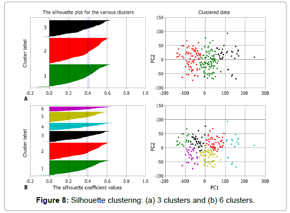
Figure 8: Silhouette clustering: (a) 3 clusters and (b) 6 clusters.

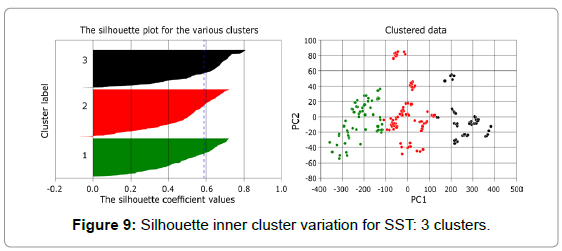
Figure 9: Silhouette inner cluster variation for SST: 3 clusters.

The calculation of the Silhouette's coefficient- (s) is made by the equation:

s = b-a / max (a, b) (7)

where a is the mean distance between a sample and all other points in the same cluster, and b is the mean distance between a sample and all other points in the next nearest cluster. From (Figures 6b and 7), it is possible to see that in the case of the Ta-SST, there are two interesting clustering possibilities: three clusters and six clusters, only the three clusters will be examined. The SST case as well presents best results for three clusters (Figures 7b and 9).

The Local Moran's I detection method

The Local Moran's I statistics (LMI), is a method for detecting local autocorrelation, also known as hot spots, by weighted comparison to its surroundings [32]. Using this methodology, after finding temporal clusters, we are able to locate areas with large SST variations in time. For that purpose, the LMI was calculated in a semi-supervised manner, based on the clusters made by the former unsupervised method, only for SST, as Ta-SST was not highly correlated with PC1 and PC2, so we could not identify specific temporal clusters.

The equation used to calculate the LMI values, follows the Environmental Systems Research Institute (ESRI) spatial statistics website (https://resources.arcgis.com) was:

(8)

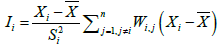
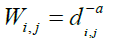
𝑋i is an attribute for feature i is an averaged value of the i feature along the specific time dimension. An average was made for each i feature split according to the clusters. The weighted matrix that was used is the powered distance matrix, which is calculated by equation (9):

(9)

is the relative distance between the i, j feature to other features, while a is a positive constant, for this research a = 1 was used, as we assume an exponential relation degradation with distance.

(10)

A low I value indicates that a chosen point has surroundings with dissimilar values. In this research, the dissimilarity is measured on the timescale, meaning the areas of negative values indicate large SST temporal variability. In addition, because it was used to find areas of interest at the sea surface during HPEs, the usage of the method was slightly different. A comparison was made between averaged LMI matrix for a certain period (as divided before), to an averaged LMI matrix of solely HPEs initial time, that occurred in the same period.

Figure 10 shows the results in terms of monthly distributions and mean fields for Ta- SST in the three-clustered segmentation. It shows that in cluster 1 (Figure 10a) high value of 77% of the HPEs that occurred in August related to this cluster. In cluster 2 (Figure 10b) the dominant months are October (63%) and September (53%). In cluster 3 (Figure 10c) there are more days of HPEs in the months of December (53%) and November (37%). Also, in clusters 1 and 3 the values are mostly negative, indicating that during HPEs at these dates the SST is higher than the air temperature and confirming that the conditions at the air-sea interface are propitious for large exchanges providing instability and potential energy for atmospheric convection processes. Cluster 2, which occurs mainly in August, has more positive values, meaning a lower thermal gradient at the air-sea interface. This indicates lower exchanges in the GOL and that the 363 sources of instability are outside the NWMED region.

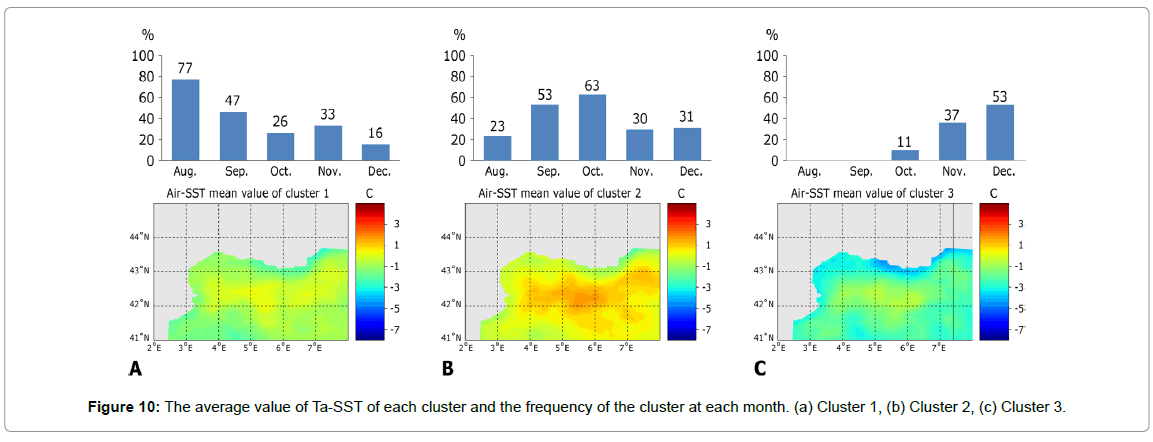
Figure 10: The average value of Ta-SST of each cluster and the frequency of the cluster at each month. (a) Cluster 1, (b) Cluster 2, (c) Cluster 3.

The low Ta-SST correlation with PC1 (0.47) and PC2 (0.1) together with uncertain temporal clustering, led us to calculate the temporal clusters for solely SST that resulted in higher correlation values (PC1: 0.88, PC2: 0.02). In Figure 11, the monthly separation clearly appears. Cluster 1 (Figure 11a), which mostly occurs in August September, has high SST values. The coldest waters (~20˚C) are located at the north-372 western corner of the domain. The absence of GOL oceanic features is related to the 373 Rhone river inputs, as will be demonstrated in the Spatial Statistics Method results. 374 Cluster 2 (Figure 11b) occurs mainly in October. The SST mean values are between 18˚C and 22˚C. The NC is clearly seen along the coast with higher SST values (~21 376 ˚C). The CC pattern can clearly be identified in the SST field with the coldest values (below 18˚C). In addition, it is interesting to see the occurrence of the Balearic front, with high temperature gradient (the thermal front suggests a general location, in contrast with the salinity front, which are more accurate as mentioned before). Cluster 3 (Figure 11c) occurs mostly during the months of November and December. As expected, during these months, the SST values are lower. The mean SST field for this cluster highlights the oceanic features mentioned before. The NC can be identified with SST of ~17 ˚C, it flows further off from the shoreline compared to the cluster representing October. To avoid confusion the names of the clusters will be written in relation to their temporal occurrence: (a) Cluster 1 (August-September): E AUT (Earlyautumn). (b) Cluster 2 386 (October): OCT. (c) Cluster 3 (November- December): L-AUT (Late-autumn).

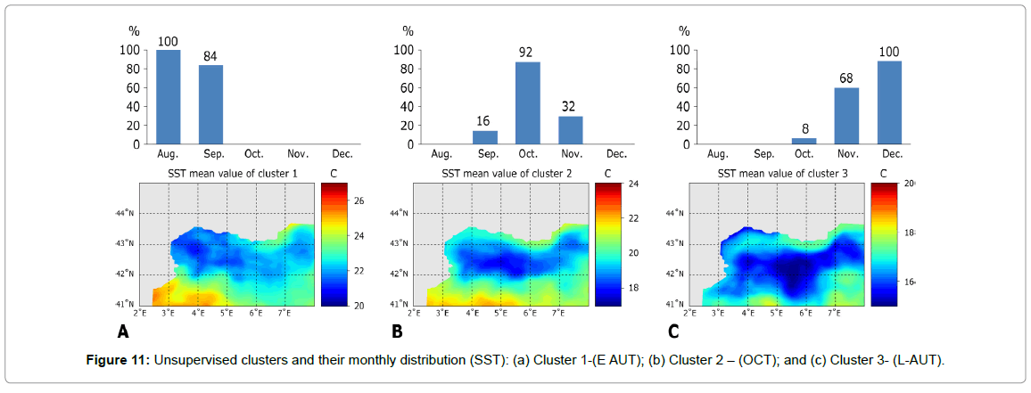
Figure 11: Unsupervised clusters and their monthly distribution (SST): (a) Cluster 1-(E AUT); (b) Cluster 2 – (OCT); and (c) Cluster 3- (L-AUT).

The LMI mean values and standard deviation for each cluster are presented in Figures 12-14 for the whole period and solely for HPEs dates. The LMI fields for the E-AUT cluster shown in Figures 12a and 12c highlight the largest SST variability related to the Rhone river spills propagating into the GOL. Due to strong stratification processes, the Rhone plume has indeed a strong signature in SST at this period. Generally, at river outlets, the circulation has a specific characterization linked to the density differences between seawater and river water. The Rhone plume under steady conditions is easily identified from the seawater surroundings, and affected from the NC. During HPEs, illustrated in Figures 12b and 12d the most significant changes occur in the same area. Moreover, after floods, the Rhone plume is less affected by the NC, and thus penetrates further into the sea. The mixing of the water masses is faster, making the plume more difficult to identify [33,34].

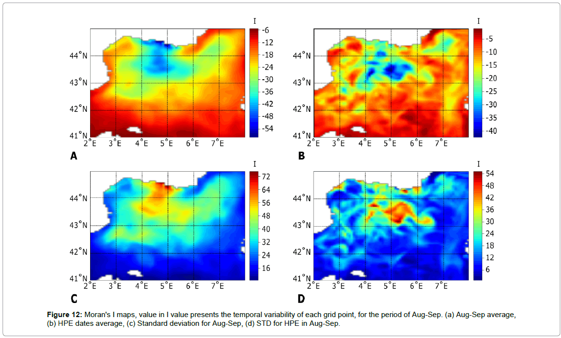
Figure 12: Moran's I maps, value in I value presents the temporal variability of each grid point, for the period of Aug-Sep. (a) Aug-Sep average, (b) HPE dates average, (c) Standard deviation for Aug-Sep, (d) STD for HPE in Aug-Sep.

Considering the OCT cluster, shown in Figures 13a and 13c, the largest variation seems to be at the center of the doming circulation pattern, which might indicate the beginning of CC intensification. Nevertheless, during HPEs, the largest variations occur at different spots, as can be seen in Figures 13b and 13d. Two main high-variability spots can be identified and related to the strong cold winds, Mistral and Tramontane. These northwesterly winds channeled in the Rhone and Aude river valley, respectively, frequently affect the GOL. The relation 412 of these strong cold winds to HPEs variations is explained by the formation of SST cold anomalies in the GOL during the preceding days of an HPE in the CV region, which in turn affects the wind (and wind stress) patterns and the atmosphere ocean fluxes, thus affecting HPEs location and intensity [10,35,36].

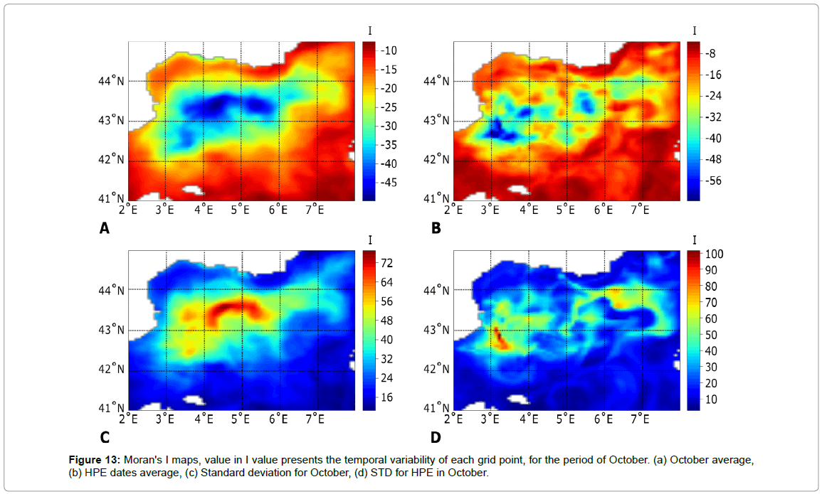
Figure 13: Moran's I maps, value in I value presents the temporal variability of each grid point, for the period of October. (a) October average, (b) HPE dates average, (c) Standard deviation for October, (d) STD for HPE in October.

For the L-AUT cluster, the LMI values are much lower, indicating a higher variability during the months of November and December(Figure 14). The most significant variation occurs along the coastline, probably because of a stronger Northern Current, which is confining the Rhone plume closer to the coastal area. A general southward displacement of the circulation pattern is noticeable as well. During HPEs the low LMI values are located at the center of the circulation pattern, indicating mixed water. Under these conditions, a convective process, and a heat and humidity transfer from deeper layers of the NWMED to the atmosphere could occur [14].

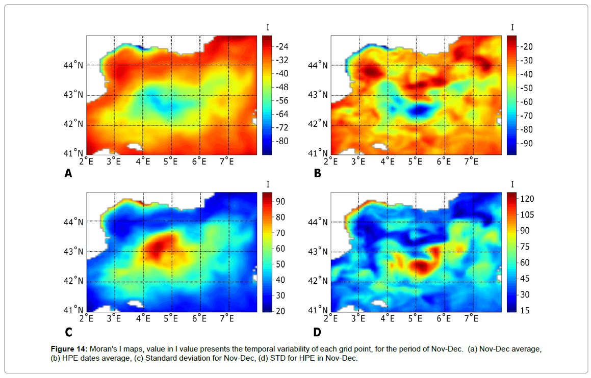
Figure 14: Moran's I maps, value in I value presents the temporal variability of each grid point, for the period of Nov-Dec. (a) Nov-Dec average, (b) HPE dates average, (c) Standard deviation for Nov-Dec, (d) STD for HPE in Nov-Dec.

This study examines the relationships between oceanic features of the GOL with HPEs in the CV region. Using spatial statistics, it demonstrates the temporal and spatial changes of the GOL waters, in general and solely during HPEs. The distribution of the HPEs and their occurrence during CSW atmospheric pattern was in agreement with the literature concerning HPEs in the CV region. The HPEs distribution found, also suggested that the majority of HPEs affecting southern France occur during October. The different relationships between the three 435 oceanographic features during the different periods (August-September, October, November-December) is observed, and suggest a general different behavior of the GOL water during initial HPEs dates, at the different observed periods. The unsupervised cluster analysis demonstrates the extent of the variation of air temperature in comparison with SST. In the Ta-SST clusters, there was not a clear segmentation between the periods of each cluster. Furthermore, the principle components had a low correlation with the Ta-SST parameter (0.57). In the SST clustering it was clear that there are three main clusters: August-September, October, and November-December and the principle components correlation with SST were high (0.89). Based on these SST clusters, it was possible to calculate a semi-446 supervised analysis and spatial statistics calculation with the LMI values, during HPEs. This analysis gives a better understanding of the variation of SST, within each period. During August-September, the Rhone River plume seems to have the greatest effect on the variation of the SST, as well as during HPEs dates. In October, the general oceanic circulation pattern starts forming, and the CC has the most significant effect on SST the variation. During HPEs, the areas with largest variation appear to be related to the Mistral and Tramontane winds, as they are located near the area where the Rhone and Aude valleys meet the coast. During November-December, the entire oceanic circulation pattern is transferred southward. The variation in SST during HPEs during this period occurs at the centre of the circulation pattern. Prior research found that the GOL water intensifies HPEs at the CV, changing their spatial location or size and has an important role on their duration. From this research it is clear that the heat and humidity exchange 459 between the GOL waters and the atmosphere above it, are temporally changing within the structure of a CSW atmospheric pattern.

The authors would like to thank the European Cooperation in Science and Technology (COST) action ES1402: Evaluation of Ocean Syntheses, which allowed for this cooperation to take place. The authors acknowledge the HyMeX database teams (ESPRI/IPSL and SEDOO/OMP) for their help in accessing the rain-gauge data.

References

- Ducrocq V, Davolio S, Ferretti R, Flamant C, Santaner VH, et al. (2016) Editorial: Introduction to the HyMeX Special Issue on 'Advances in understanding and forecasting of heavy precipitation in the Mediterranean through the HyMeX SOP1 field campaign'. QJR Meteorol Soc 142: 1-6.
- Delrieu G, Ducrocq V, Gaume E, Nicol J, Payrastre O, et al. (2005) The catastrophic flash-flood event of 8-9 September 2002 in the Gard region, France: A first case study for the Cévennes-Vivarais Mediterranean Hydrometeorological Observatiory. Journal of Hydrometeorology 6: 34-52.
- Vinet F (2008) Geographical analysis of damage due to flash floods in southern France: The cases of 12-13 November 1999 and 8-9 September 2002. Applied Geography 28: 323-336.
- Bresson E, Ducrocq V, Nuissier O, Ricard D, And DS, et al. (2012) Idealized numerical simulations of quasi-stationary convective systems over the North-western Mediterranean complex terrain. QJR Meteorol Soc 138: 1751-1763.
- Ducrocq V, Braud I, Davolio S, Ferretti R, Flamant C, et al. (2014) HYMEX-SOP1-The Field Campaign Dedicated to Heavy Precipitation and Flash Flooding in the North-western Mediterranean. BAMS 95: 1083-1100.
- Pastor F, Estrela MJ, Penarrocha P, Millan MM (2001) Torrential rains on the spanish Mediterranean coast: Modelling the effect of the sea surface temperature. J Appl Meteorol 40: 1180-1195.
- Lebeaupin-Brossier C, Ducrocq V, Giordani H (2006) Sensitivity of torrential rain events to the sea surface temperature based on high-resolution numerical forecasts. Journal of Geophysical Research 111: 12110.
- Romero R, Ramis C, Homar V (2015) On the severe convective storm of 29 October 2013 in the Balearic Islands: observational and numerical study. Quart J Roy Meteorol Soc 141: 1208-1222.
- Berthou S, Mailler S, Drobinski P (2014) Prior history of Mistral and Tramontane winds modulates heavy precipitation events in southern France. Tellus A 66: 24064.
- Lebeaupin-Brossier C, Drobinski P, Béranger K, Bastin S, Orain F (2013) Ocean memory effect on the dynamics of coastal heavy precipitation preceded by a mistral event in the north-western Mediterranean. QJR Meteorol Soc 139: 1583-1597.
- Millot C, Taupier-Letage I (2005) Circulation in the Mediterranean Sea. Handbook of Environmental Chemistry 5: 29-66.
- Marshall J (1999) Open-ocean convection: Observations, theory and models. Reviews of Geophysics 37: 1-64.
- Houpert L, Testor P, Durrieu DX, Somot S, D'Ortenzio F, et al. (2015) Seasonal cycle of the mixed layer, the seasonal thermocline and the upper-ocean heat storage rate in the Mediterranean Sea derived from observations. Progress in Oceanography 132: 333-352.
- Madec G, Chartier M, Delecluse P, Crepon M (1991) A three-dimensional numerical study of deep water formation in the north-western Mediterranean Sea. J Phys Oceanogr 21: 1349-1371.
- Madec G, Lott F, Delecluse P, Crepon M (1996) Large-scale preconditionning of deep-water formation in the north-western Mediterranean Sea. J Phys Oceanogr 26: 1393-1408.
- Leaman KD, Schott A (1991) Hydrographic structure of the convection regime in the Gulf of Lions: Winter 1987. J Phys Oceanogr 21: 575-598.
- Hamon M, Beuvier J, Somot S, Lellouche JM, Greiner E, et al. (2016) Design and validation of MEDRYS, a Mediterranean Sea reanalysis over the period 1992-2013. Ocean Science 12: 577-599.
- Schroeder K, Garcia-Lafuente J, Josey SA, Artale V, Nardelli BB, et al. (2012) Circulation of the Mediterranean Sea and its Variability. The Climate of the Mediterranean Region. 12: 187-256
- Alberola C, Millot C, Font J (1995) On the seasonal and mesoscale variabilities of the Northern Current during the PRIMO-0 experiment in the western Mediterranean Sea. Oceanologica ACTA 18: 163-192.
- Pascual A, Gomis D (2002) Use of surface data to estimate geostrophic transport. Journal of atmospheric and oceanic technology 20: 912-926.
- Lopez Garcia Mj, Millot C, Font J, Garcia-Ladona E (1994) Surface circulation variability in the Balearic Basin. Journal of Geophysical Research 99: 3285-3296.
- Font J, Salat J, Tintore J (1988) Permanent features of the circulation in the Catalan sea. Oceanologica
- Di-Luca A, Flaounas E, Drobinski P, Lebeaupin-Brossier C (2014) The Atmospheric component of the Mediterranean Sea water budget in a WRF multi-physics ensemble and observations. Clim Dyn 43: 2349-2375.
- Ricard D, Veronique D, Auger L (2012) A climatology of the mesoscale environment associated with heavily precipitating events over a Northwestern Mediterranean Area. J Appl Meteorol Climatol 51: 468-488.
- Kalnay E, Kanamitsu M, Kistler R, Collins, W, Deaven D, et al. (1996) The NCEP/NCAR 40-year reanalysis project. Bull Amer Meteor Soc 77: 437-470.
- Beuvier J, Lebeaupin BC, Beranger K, Arsouze T, Bourdalle-Badie R, et al. (2012) MED12 oceanic component for the modeling of the regional Mediterranean Earth System. Mercator Ocean 30 Quaterly Newsletter 46: 60-66.
- Madec G (2008) NEMO ocean engine. Note du Pole de modelisation. Institu Pierre-Simon Laplace. Paris.
- Lellouche JM, Galloudec O, Drévillon M, Régnier C, Greiner E, et al. (2013) Evaluation of global monitoring and forecasting systems at Mercator Ocean. Ocean Sci 9: 57-81.
- Reynolds RW, Smith TM, Liu C, Chelton DB, Casey KS, et al. (2007) Daily high-resolution blended analyses for sea surface temperature. J Climate 20: 5473-5496.
- Rousseeuw PJ (1987) Silhouettes: A graphical aid to the interpretation and validation of cluster analysis. J Comput Appl Math 20: 53-65.
- Anselin, L (1995) Local Indicators of Spatial Association-LISA. Geographical Analysis 27: 93-115.
- Broche P, Devenon JL, Forget P, De-Maistre JC, Naudin JJ, et al. (1998) Experimental study of the Rhone plum. Part 1: Physics and dynamics. Oceanologica ACTA.21: 725-738.
- Estournel C, Broche P, Marsaleix P, Devenon JL, Auclair F, et al. (2001) The Rhone river plume in unsteady conditions: Numerical and experimental results. Estuarine Coastal and Shelf Science 53: 25-38.
- Berthou S, Mailler S, Drobinski P, Arsouze T, Bastin S, et al. (2015) Sensitivity of an intense rain event between atmosphere-only and atmosphere-ocean regional coupled modles. QJR Meteorol Soc 141: 258-271.
- Lebeaupin-Brossier C, Ducrocq V, Giordani H (2008) Sensitivity of three Mediterranean heavy rain events to two different sea surface fluxes parameterizations in high-resolution numerical modeling. ‎J Geophys Res 113: 21109.
Citation: Robins L, Anna B, Marie D, Jonathan B, Cindy LB, et al. (2018) Temporal Variability of Sea Surface Temperature Patterns in the Gulf of Lions During Heavy Precipitation Events in The Cevennes-Vivarais Region. J Earth Sci Clim Change 9: 469. DOI: 10.4172/2157-7617.1000469
Copyright: © 2018 Robins L, et al. This is an open-access article distributed under the terms of the Creative Commons Attribution License, which permits unrestricted use, distribution, and reproduction in any medium, provided the original author and source are credited.
Select your language of interest to view the total content in your interested language
Share This Article
Recommended Journals
Open Access Journals
Article Tools
Article Usage
- Total views: 6640
- [From(publication date): 0-2018 - Nov 12, 2025]
- Breakdown by view type
- HTML page views: 5586
- PDF downloads: 1054