Research Article Open Access
Environmental Influences on the Abundance of Dominant Fishes in a Very Shallow Tropical Coastal Lagoon in Northwestern Yucatan Peninsula, Mexico
José Luis Bonilla-Gómez1*, Maribel Badillo2, Korynthia López3, Alfredo Gallardo2, Carmen Galindo2, Daniel Arceo2 and Xavier Chiappa-Carrara2
1Department of Marine Sciences and Limnology, National Autonomous University of Mexico, Mexico D. F., Mexico
2UNAM-Sisal, Faculty of Science, National University of Mexico, Sisal, Yucatan, Mexico
3UNAM-Sisal, Faculty of Chemistry, National Autonomous University of Mexico, Sisal, Yucatan, Mexico
- *Corresponding Author:
- José Luis Bonilla-Gómez
Department of Marine Sciences and Limnology
National Autonomous University of Mexico, Circuito Exterior S/N
Ciudad Universitaria, Mexico DF, 04510, Mexico
Tel: (52) 999-1813611
E-mail: jose.bonilla@comunidad.unam.mx
Received date: January 12, 2013; Accepted date: February 18, 2013; Published date: February 22, 2013
Citation: Bonilla-Gómez JL, Badillo M, López K, Gallardo A, Galindo C, et al. (2013) Environmental Influences on the Abundance of Dominant Fishes in a Very Shallow Tropical Coastal Lagoon in Northwestern Yucatan Peninsula, Mexico. J Marine Sci Res Dev 3:118. doi:10.4172/2155-9910.1000118
Copyright: © 2013 Bonilla-Gómez JL, et al. This is an open-access article distributed under the terms of the Creative Commons Attribution License, which permits unrestricted use, distribution, and reproduction in any medium, provided the original author and source are credited.
Visit for more related articles at Journal of Marine Science: Research & Development
Abstract
Spatial-seasonal patterns of six abundant fishes were analyzed in La Carbonera, a lagoon on the northwestern coast of the Yucatan peninsula, Mexico; between April 2009 and May 2010, via non-parametric multivariate analysis. The null hypothesis tested was that no differences existed in the overlapping of the abundance of fish species among the lagoon defined by types of habitats (channel, seagrass, mangrove and hypersaline), and by three climatic seasons (dry, rainy, and north winds). Significant differences were found in the environmental variables between climatic season and the types of habitat, except for the temperature and pH. Result of the multidimensional scaling suggests a significant difference in habitats with characteristics of channel and presence of mangrove. The redundancy analysis showed that depth and salinity were the best related to species abundance. Oxygen and temperature made an additional significant contribution to the canonical model, it was strongly related to the north winds season, due to the fact that the strong winds, which can last a week, increase the oxygen content of the water but decrease the temperature. Relative abundances were strongly associated with depth (dry; r=0.76), salinity (rainy; r=0.83) and oxygen (north winds; =-0.80). Results suggest that the different habitats are used as feeding zones; and that during the dry season, there was a overlapping in abundance of species. Thus, information proposed protection strategies in this season to contribute to fish biodiversity conservation in a valuable area of Yucatan Peninsula.
Keywords
Spatial-seasonal patterns; Multidimensional scaling; Redundancy analysis; La Carbonera lagoon
Introduction
The Yucatan peninsula has numerous coastal lagoons, where their structure and function are being modified by wastewater discharge, groundwater pumping, and land use changes [1]. They are generally standing water with the calm hydrodynamics that are essential for many juvenile and adult fish [2]. Knowledge of the response of these fishes to changes in environmental conditions will contribute to our understanding of the potential effects of anthropogenic impacts on estuarine fish species [3].
The habitat patterns; such as mangrove and seagrass can be viewed as a reference of an assemblage of the ichthyofauna for tropical karstic lagoons [4]. In Yucatan, information is also available about fish assemblages in tropical coastal systems influenced by freshwater inputs [5,6] and fish assemblages in a coastal hypersaline lagoon [7]. There are many studies of fish assemblages in temperate systems [8], but little information exists about tropical karstic estuarine systems, particularly along the northwestern coast of the Yucatan peninsula. Several species, such as: Lagodon rhomboides (pinfish), Sphoeroides testudineus (checkered puffer), Mugil curema (white mullet), Chriodorus atherinoides (hardhead halfbeak), Eucinostomus argenteus (silver mojarra) and Eucinostomus gula (Jenny mojarra) have been already described as “abundant” in the coastal lagoons of Yucatan, contributing with more than 50% considering and analysis of the entire fish assemblage caught with seine net and their importance value index [5,9]. However, few studies analyze the population dynamics of wetland fishes for possible correlations with hydrological variables [10].
In terms of the climatic seasons, the Yucatan peninsula has three marked seasons annually: dry, rainy and north winds [9,11,12]. In small karstic coastal lagoons of the Yucatan, which are a typical system along this coast, the dry season like the hottest reduced and altered the habitat available for fish species [13]. La Carbonera, a karstic coastal lagoon, is a transitional environment between a karstic land and a marine habitat with high environmental variability over short time scales, and this lagoonal system is important for local fisheries and as bird habitat (e.g., flamingos Phoenicopterus ruber). The present study investigates extreme shallowness of the system along with the susceptibility of environmental changes, the presence of an overlapping between the abundance of six abundant population of fish among the La Carbonera lagoon defined by four habitat types (channel, seagrass, mangrove and hypersaline), and about the climatic season basis (dry, rainy, and north winds).
Materials and Methods
Study area
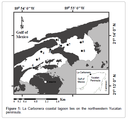
La Carbonera coastal lagoon lies on the northwestern Yucatan peninsula, Mexico (21°13'-21°14' N; 89°52'-89°54' W; Figure 1). It is connected to the sea by a channel formed in 1988 by Hurricane Gilbert, and is fringed with Rhizophora mangle stands and a sand barrier. The lagoon is very shallow (average depth 0.5 m) and covers an area of ~16.5 km2. It is a very low karstic marine-biogenic littoral [14]. Freshwater input is restricted to underground seeps and rainfall. There is a cenote (sinkhole) in the southern part of the lagoon, in a patch of mangroves. There are three climatic seasons in the zone: dry (D; March-June), rainy (R; July-October) and north winds (NW; November-February) [11]. The system presents three different types of vegetation: mangroves, seagrass, and spring with bushes patch called colloquially “petenes”; and the same karstic substratum throughout [15] with three types of sediments: sandy, rocky bed and muddy. Hence, four types of habitat were identified in situ in the nine stations according to [16], which are based on substrate, salinity, vegetation: hyperhaline (H), seagrass (S), channel (C), and mangrove (M) (Table 1).
Sampling and environmental data
Fourteen monthly sampling including fish and physical variables were performed between April 2009 and May 2010 during the three climate seasons (D, R, and NW) in nine sampling stations distributed in different types of habitats (H, S, C, and M). We recorded water temperature (°C), salinity, pH, dissolved oxygen (mg/L) and total dissolved solids (TDS, mg/L) at each sampling station (measured at 30 cm depth) with a Yellow Springs Instrument (YSI), model 556 MPS. Wind speed (km/h) and direction was determined with an anemometer, Sper Scientific 850070. Depth (cm) was recorded at each sampling station.
Juveniles of L. rhomboides, S. testudineus, M. curema, C. atherinoides, E. argenteus, and E. gula were caught monthly with a beach seine net (40 m long×1 m depth×1.27 cm stretch mesh size; Mexican government permit No. DOPA/04031/310510.1940). The sampling area was 400 m2, with one sample per station; the net was cast once in each site for each month. All sites were sampled within a 6 h period during high tide on the same day. Specimens were euthanized in ice slurry, preserved in formaldehyde (4%) and transported to the laboratory, where they were identified and weighed (± 0.01 g precision). All the six species were considered euryhaline marine.
Data Analysis
The environmental variable data collected in the sampling stations were grouped per type of habitats (C, S, H, and M; Table 1), and the monthly data were performed per climate seasons (D, R, and NW). A factorial two-way variance analysis (ANOVA) assessed spatial and seasonal differences in the environmental data and the interaction between habitat and season, having previously verified the assumptions of normality (Kolmogorov Smirnov) and homogeneity of variance (Bartlett and Cochran) [17]. Analyses used STATISTICA 7.0 (StatSoft Inc.).
| Station | Habitat | Substrate | Depth (cm) | Temp. (ºC) | Salinity | O2 (mg/L) | TSD (mg/L) | pH |
|---|---|---|---|---|---|---|---|---|
| 1 | Channel | Rocky, Sandy | 56.6 ± 24.7 | 28.8+4.4 | 37.7 ± 4.6 | 7.5 ± 1.7 | 30.8 ± 9.9 | 8.2 ± 0.2 |
| 2 | Mangrove (60) | Sandy | 39.9 ± 24.5 | 27.4 ± 3.1 | 36.9 ± 5.2 | 6.1 ± 1.5 | 30.7 ± 9.4 | 8.1 ± 0.2 |
| 3 | Channel | Muddy | 72.6 ± 33.0 | 27.3 ± 3.8 | 33.2 ± 3.5 | 6.4 ± 1.6 | 25.1 ± 13.5 | 8.2 ± 0.3 |
| 4 | Seagrass (80) | Sandy, Muddy | 27.7 ± 12.0 | 28.8 ± 3.8 | 30.3 ± 6.4 | 7.6 ± 1.6 | 24.1 ± 11.5 | 8.2 ± 0.3 |
| 5 | Hyperhaline | Muddy | 35.1 ± 13.4 | 29.0 ± 4.0 | 31.3 ± 14.2 | 7.6 ± 2.3 | 24.4 ± 12.5 | 8.2 ± 0.3 |
| 6 | Channel | Sandy | 57.1 ± 17.0 | 29.8 ± 4.2 | 28.8 ± 4.6 | 7.9 ± 1.1 | 24.0 ± 13.7 | 8.2 ± 0.3 |
| 7 | Channel | Sandy | 63.5 ± 41.2 | 27.9 ± 2.7 | 34.8 ± 5.0 | 5.9 ± 1.8 | 29.9 ± 11.2 | 8.0 ± 0.4 |
| 8 | Hyperhaline | Sandy | 41.5 ± 10.5 | 28.8 ± 3.4 | 38.1 ± 8.9 | 7.3 ± 1.6 | 32.3 ± 12.1 | 8.2 ± 0.2 |
| 9 | Mangrove (70) | Muddy | 32.6 ± 12.0 | 30.3 ± 4.9 | 34.1 ± 6.2 | 7.5 ± 1.9 | 34.6 ± 8.9 | 8.2 ± 0.2 |
Table 1: Characteristics of the different sampling stations, type of habitats (based on substrate, salinity, vegetation observed in situ) and mean values (± standard deviation) of the environmental variables present in each sampling stations. % refers to the percentage cover in each habitat.
Multivariate statistical analyses of spatial-seasonal fish data used the PRIMER v.6 and Permanova add program [18]. Similarities between samples were computed by a Bray-Curtis dissimilarity matrix using fish species abundances with a Log (x+1) transformed data; they were graphically represented by cluster analysis (using group-average linking based on Bray-Curtis similarities), which was used to define groups of site preferences and ordination plots by species (using total abundances). A similarity matrix was used to generate a non-metric multidimensional scaling (MDS) ordination [19]. MDS constructs a 2-dimensional ordination in a manner that best represents relationships among samples in a similarity matrix [20,21]. In ordination plots, the relative distance between points reflects the similarity of species abundance in those samples. MDS was verified by taking into account the value of stress: low values (<0.1) suggest good separations among the groups, while higher values (>0.2) indicate that the results should be interpreted with caution [21]. An analysis of similarity (ANOSIM) was performed between the fish of each habitat and climatic seasons [22], with a non parametric test that uses a Bray-Curtis similarity matrix with abundance data. This procedure consists of a statistical test (R), which is analogous to an ANOVA. The null hypothesis tested was that no differences existed between the fish abundances in the different type of habitats.
Detrended Correspondence Analysis (DCA) on species data assessed the length of the gradients [23]; these were 1.12 for the first axis and <2 for the rest of the axes, suggesting a linear response model [24]. Based thereon, Redundancy Analysis (RDA) examined the relationships between the environmental variables of the lagoon and between the species abundance and sampling stations, using the program CANOCO for Windows 4.5 [25]. RDA computations were performed on log-transformation [y´=log (a*y+b)] and centered by species (no centering for samples was performed). Scaling focused on inter-sample distances and there was no post-transformation of species scores. The RDA used the correlation matrix option, and scaling was conducted on a correlation triplot ordination. The significance of each environmental variable was tested through 499 unrestricted Monte Carlo permutations.
Results
Environmental conditions
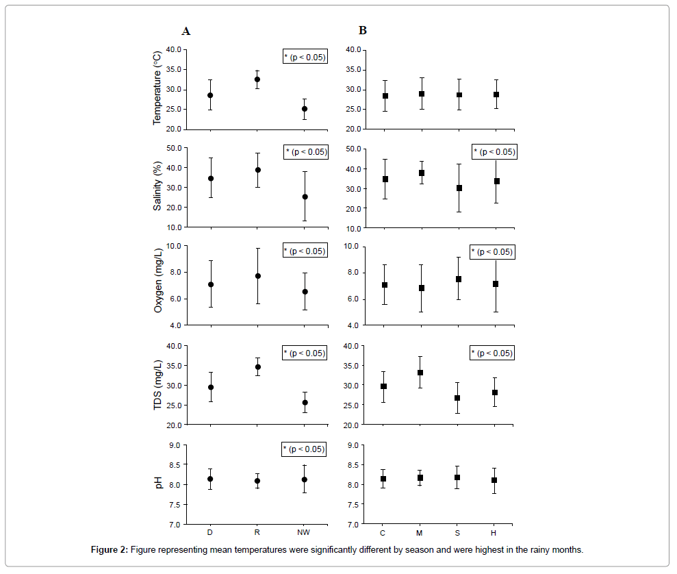
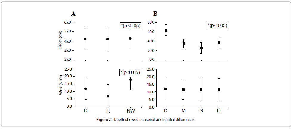
Mean temperatures (Figure 2) were significantly different by season (Table 2), and were highest in the rainy months; particularly registered in August (34.2°C) and October (32.6°C), and were lowest when north winds prevailed, with a minimum of 20.3°C registered in February. No spatial (per habitat) variation was observed (p>0.05). Mean salinity was 35.1 (range 3.8-52.7) in the sampling period; seasonal and spatial variation were significant different (p<0.05; Table 2) and were higher in M (Figure 2). Dissolved oxygen varied significantly with season and with the habitats, especially in S, with highest and lowest mean values occurring in August and September (Figure 2). Test supported Development (TSD) and pH both indicated significant variations with the season values ranging from 27 to 35 mg/L and 8.02 to 8.19 respectively. TDS showed spatial differences, being higher in M (p<0.05), but the pH was no different between habitats (Figure 2). Depth showed seasonal and spatial differences, and were higher in C (Figure 3) being shallow in the dry season and, spatially, being shallowest in stations 1, 4 and 5 and deepest in stations 3 and 7 (Table 1). Wind velocity varied with season variations (Figure 3).
| Variables/Effects | S. S. | D. F. | M. S. | F | p |
|---|---|---|---|---|---|
| Temperature | |||||
| Season | 786.53 | 2 | 393.27 | 55.79 | *0.0000 |
| Habitat | 8.52 | 3 | 2.84 | 0.40 | 0.7513 |
| Season-Habitat | 13.09 | 6 | 2.18 | 0.31 | 0.9309 |
| Salinity | |||||
| Season | 3711.0 | 2 | 1855.5 | 30.261 | *0.0000 |
| Habitat | 823.8 | 3 | 274.6 | 4.478 | *0.0052 |
| Season-Habitat | 624.8 | 6 | 104.1 | 1.698 | 0.1279 |
| Dissolved oxygen | |||||
| Season | 18.281 | 2 | 9.140 | 2.943 | 0.0568 |
| Habitat | 4.387 | 3 | 1.462 | 0.471 | 0.7032 |
| Season-Habitat | 4.261 | 6 | 0.710 | 0.229 | 0.9665 |
| TDS | |||||
| Season | 1124.68 | 2 | 562.34 | 4.5829 | *0.0125 |
| Habitat | 640.65 | 3 | 213.55 | 1.7404 | 0.1637 |
| Season-Habitat | 445.35 | 6 | 74.22 | 0.6049 | 0.7258 |
| pH | |||||
| Season | 0.129 | 2 | 0.065 | 0.94 | 0.3948 |
| Habitat | 0.093 | 3 | 0.031 | 0.45 | 0.7175 |
| Season-Habitat | 0.238 | 6 | 0.040 | 0.57 | 0.7503 |
| Depth | |||||
| Season | 481.7 | 2 | 240.9 | 0.4413 | 0.6443 |
| Habitat | 28173.1 | 3 | 9391.0 | 17.2063 | *0.0000 |
| Season-Habitat | 5458.6 | 6 | 909.8 | 1.6669 | 0.1357 |
| Wind velocity | |||||
| Season | 1565.84 | 2 | 782.92 | 5.3511 | *0.0060 |
| Habitat | 29.54 | 3 | 9.85 | 0.0673 | 0.9772 |
| Season-Habitat | 579.72 | 6 | 96.62 | 0.6604 | 0.6817 |
Table 2: Results of the factorial two-way ANOVA to test spatial and seasonal significant differences (*; p<0.05) in the environmental variables registered.
Spatial and Seasonal Variations in Fish Abundance
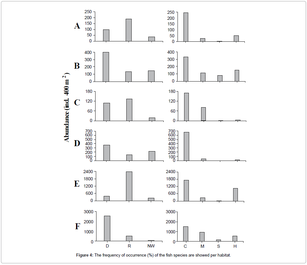
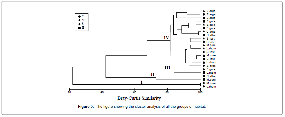
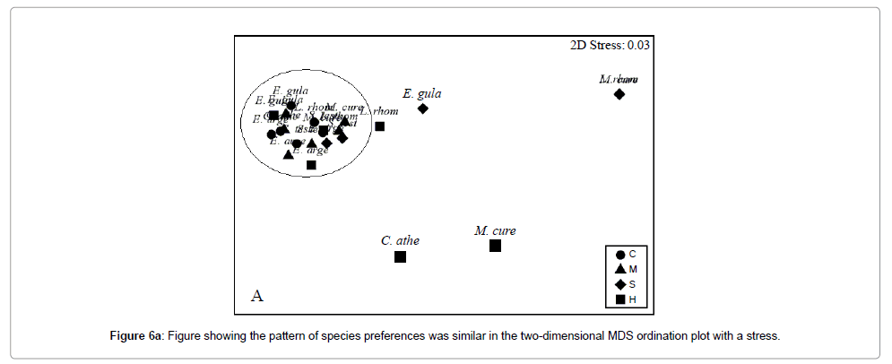
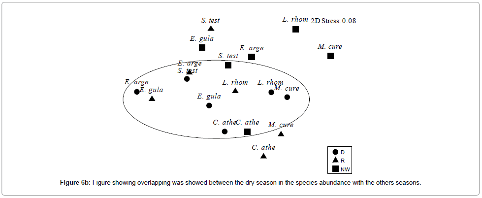
A total of 8370 specimens were captured and each species occurred in all sampling stations, except that C. atherinoides was never caught in station 4 with a sea grass habitat type (Table 3, Figure 4). Also, C. atherinoides, M. curema and E. argenteus were not found in some months, whereas L. rhomboides, S. testudineus and E. gula occurred in all months. Most species were most abundant in the dry season, but M. curema and E. gula were more abundant in the rainy season (Figure 4). Cluster analysis showed four groups of habitat (sampling stations) preferences with a similarity level between groups (Bray- Curtis similarity) of 22 to 82% (Figure 5). Group I; which included the habitat S, and was distinct from other groups, showing 22% similarity. Sphoeroides testudineus occurred in the group IV, L. rhomboides and C. atherinoides in group I, III and IV; M. curema in groups I, II and IV; E. gula in groups III and IV; and while E. argenteus in group IV. The fish populations were most frequent in deeper sites, high salinities in the lagoon and preference by Channel and mangrove habitats. This pattern of species preferences was similar in the two-dimensional MDS ordination plot with a stress of 0.08 and 0.03, which is a good representation of the diagram (Figure 6a). Also an overlapping was showed between the dry season in the species abundance with the others seasons (Figure 6b). The one-way ANOSIM with 999 permutations indicated significant differences in the composition of fish abundance between the different habitats (r=354, p<0.05).
| Species | Family | N | %D | %B | Frequency of occurrence (%) | ||||||
|---|---|---|---|---|---|---|---|---|---|---|---|
| Habitat | Climatic season | ||||||||||
| Channel | Mangrove | Seagrass | Hypersaline | Dry | Rainy | North | |||||
| E. argenteus | Gerreidae | 3079 | 36.68 | 7.39 | 5.32 | 1.87 | 0.73 | 2.79 | 86.45 | 11.33 | 2.22 |
| E. gula | Gerreidae | 3094 | 36.97 | 7.66 | 7.19 | 7.88 | 30.55 | 8.70 | 15.04 | 77.22 | 7.74 |
| C. atherinoides | Hemiramphidae | 699 | 8.35 | 10.88 | 3.68 | 5.60 | 0.73 | 0.28 | 42.90 | 22.71 | 34.38 |
| M. curema | Mugilidae | 252 | 3.01 | 3.15 | 14.60 | 2.42 | 0.00 | 1.00 | 45.23 | 47.72 | 7.05 |
| L. rhomboides | Sparidae | 569 | 6.80 | 8.80 | 37.00 | 18.80 | 8.73 | 57.30 | 64.11 | 29.16 | 6.73 |
| S. testudineus | Tetraodontidae | 686 | 8.20 | 63.13 | 32.21 | 63.44 | 59.27 | 29.93 | 63.67 | 13.27 | 23.06 |
Table 3: Total of individuals (N), relative density (D 400 m2) and the relative biomass (B 400 m2) found during the period of study (April 2009-May 2010). The frequency of occurrence (%) of the fish species are showed per habitat (spatial variation) and per climatic seasons (temporal variation), both analysis with independient data. (NW=Norths winds).
Effect of Environmental Variables on Spatial-seasonal Variation of Fishes
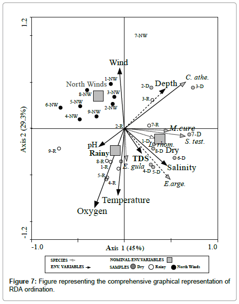
RDA yielded a first canonical ordination axis explaining 23.4% of the variance of species data and 45% of the species-environment relationship (Table 4). This axis had a very high species-environment correlation. Joint examination of canonical coefficients and inter-set correlations helped to identify this first axis reflecting a salinity and depth gradient (Table 4). The second canonical axis explained less variation (15.2% of species data and 29.3% of species-environment relation) but had also a high species-environment correlation. This axis can be clearly identified with a negative gradient of oxygen and temperature. Through a triplot, a comprehensive graphical representation of RDA ordination examined the number of samples, species and environmental variables reflected the salinity and depth arrow and the first canonical ordination axis a high correlation between them (Figure 7). The pH and TDS are also correlated with the first axis. The arrows representing wind, temperature and oxygen forms an acute angle with the second ordination axis, reflecting the high correlation between them. Projections of centroids of the nominal variable used to represent climatic seasons show clearly that this variable has a very low discriminatory value due to the position of the centroids of its classes near the origin of the axes. However, during the north winds season, a group of samples was clearly shown. During the dry season, the species were highly correlated among them, and with depth, salinity, and TDS. Meanwhile, M. curema, S. testudineus, L. rhomboides, and E. argenteus were highly correlated mainly to salinity and were associated to the dry season (included as dummy variable), in relation with the first canonical axis (45%). However, E. gula showed a highly correlation with the temperature and an inverse relation with the wind velocity, and C. atherinoides showed a high relation with depth and an inverse relation with the pH (Figure 7).
| Summary of the ordination axes | 1 | 2 | 3 | 4 |
|---|---|---|---|---|
| Eigenvalues | 0.234 | 0.152 | 0.089 | 0.033 |
| Species-environment correlations | 0.789 | 0.800 | 0.653 | 0.616 |
| Cumulative percentage variance | ||||
| of species data | 23.4 | 38.6 | 47.5 | 50.8 |
| of species-environment relation | 45.0 | 74.3 | 91.3 | 97.6 |
| Canonical coefficients for standardized variables and inter-set correlations of environmental variables with species axes | Canonical coefficient | Inter-set correlation | ||
| Axis 1 | Axis 2 | Axis 1 | Axis 2 | |
| Depth | 0.437 | 0.434 | 0.345 | 0.347 |
| Oxygen | -0.319 | -0.845 | -0.252 | -0.676 |
| Temperature | -0.068 | -0.718 | -0.054 | -0.574 |
| Salinity | 0.458 | -0.401 | 0.361 | -0.321 |
| pH | -0.274 | -0.193 | -0.216 | -0.154 |
| TDS | 0.186 | -0.265 | 0.147 | -0.212 |
| Wind | -0.056 | 0.653 | -0.044 | 0.522 |
| Dry season | 0.720 | -0.216 | 0.569 | -0.173 |
| Rainy season | -0.191 | -0.447 | -0.151 | -0.358 |
| North winds season | -0.529 | 0.663 | -0.418 | 0.530 |
Table 4: Summary of redundancy analysis.
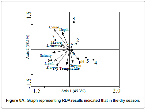
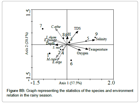
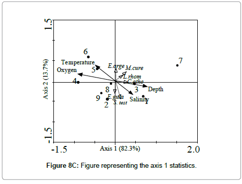
In the triplots of species, samples, and environmental variables (Figure 8), the distance between sampling stations (focused in samples) in the plot does not reflect the Euclidean distances between them due to scaling used, basically focused on species correlations. The projections of species, environmental variables and sampling stations on canonical axes is a way to understand main environmental variables associated to each group of climatic season. RDA results indicated that in the dry season (Figure 8a), axis 1 explained about 45.3% and axis 2 explained 38.1% of the relationship between species and environment. In the rainy season, axis 1 explained 57.5% and axis 2 explained 20.1% of the species and environment relation (Figure 8b). When north winds prevailed, axis 1 explained 82.3% and axis 2 explained 13.7% (Figure 8c). Depth showed the vector of length best correlated in the dry season with axis 2, r=0.76 and an inflation factor of 1.37 (Table 5), followed by salinity, which was best correlated with axis 1, r=-0.63 and an inflation factor of 1.67. In the dry season, abundance of C. atherinoides was highly correlated with depth; E. gula and E. argenteus were highly correlated with salinity and temperature and abundant at stations 8 and 9, and were inversely correlated with S. testudineus and station 2. M. curema and L. rhomboides were inversely correlated with pH and preferred station 7. No preferences or correlations were observed for station 3, the deepest station (Figure 8a).
In the rainy season, the salinity had the vector length best correlated with axis 1, r=0.83 and an inflation factor of 1.63 (Table 5); temperature was the second best correlated with axis 1, r=0.63 (Figure 8b). Lagodon rhomboides, E. gula and S. testudineus were highly correlated with depth and inversely with temperature and oxygen, and correlated with station 2. Abundance of M. curema and E. argenteus was highly correlated with stations 2 and 4, and inversely correlated to TDS and pH. Chriodurus atherinoides was correlated with station 8. There were no preferences or direct correlation to environmental variables for stations 1, 6, and 7.
| Season | Variables | Inflation factor | Canonical coeff.-axis 1 | Canonical coeff.-axis 2 | Correlation (r) species-axis 1 | Correlation (r) species-axis 2 |
|---|---|---|---|---|---|---|
| Dry | Depth | 1.37 | -0.341 | 0.867 | -0.27 | 0.76 |
| Oxygen | 9.97 | 0.155 | -0.689 | 0.13 | -0.60 | |
| Temperature | 6.75 | -0.134 | -0.775 | -0.11 | -0.68 | |
| Salinity | 1.67 | -0.786 | -0.173 | -0.63 | -0.15 | |
| pH | 3.67 | 0.433 | -0.531 | 0.35 | -0.47 | |
| TDS* | - | - | - | - | - | |
| Wind* | - | - | - | - | - | |
| Rainy | Depth | 2.35 | -0.376 | -0.011 | -0.34 | -0.01 |
| Oxygen | 2.99 | 0.449 | -0.329 | 0.41 | -0.33 | |
| Temperature | 3.72 | 0.696 | -0.266 | 0.63 | -0.26 | |
| Salinity | 1.63 | 0.911 | 0.258 | 0.83 | 0.26 | |
| pH | 1.60 | 0.022 | 0.449 | 0.02 | 0.45 | |
| TDS | 1.94 | 0.362 | 0.747 | 0.33 | 0.74 | |
| Wind* | - | - | - | - | - | |
| North winds | Depth | 1.64 | 0.711 | -0.265 | 0.70 | -0.22 |
| Oxygen | 2.19 | -0.821 | 0.339 | -0.80 | 0.28 | |
| Temperature | 1.50 | -0.433 | -0.748 | -0.42 | 0.61 | |
| Salinity | 2.18 | 0.390 | -0.643 | 0.38 | -0.53 | |
| pH* | - | - | - | - | - | |
| TDS* | - | - | - | - | - | |
| Wind* | - | - | - | - | - |
Table 5: Results of the inflation factor, canonical coefficients and the best correlation (r) using redundancy analysis (RDA). The table show the environmental variables per climatic season.
During the season of north winds, fish abundance was inversely correlated to oxygen, it showed a best correlation with axis 1 (r=-0.80 with inflation factor of 2.19) (Table 5), followed by the depth vector length with a best correlated with axis 1 (r=0.70) (Figure 8c). Projections of abundance of all species on canonical axes and environmental factors showed correlated with lagoon depth and salinity, and inversely correlated to oxygen and temperature, including their prolongations in the direction opposite to the arrowhead. The species showed correlation with stations 1 and 3 and inversely with station 2, 8, and 9. E. gula and E. argenteus are not correlated with environmental variables, but show a clear high correlation with the second axis. Station 7 did not show direct correlations with the environmental variables.
Discussion
Spatial and temporal differences of environmental variables
In the lagoon system of La Carbonera, high salinity and temperature were found in the dry season. One exception corresponds to October 2009, which was an atypical month since high temperatures and low precipitation led to the salinity increase during the rainy season instead the usual dilution of the rainfall that is normally observed. A salinity peak (~50) in October 2009 was reported by [26], which is different with the lowest salinity (~15) found in December 2009 at the end of the rainy season. Both salinity and temperature gradually decrease until the lowest values were registered in the north winds season, following the general pattern found also by [16] in another hypersaline coastal system on the northeastern coast of the Yucatan peninsula. The presence of northerly winds, usually colder and faster, is important in the spatial distribution of the environmental features of this shallow system. This is especially true when considering the dissolved oxygen values, which increase due to turbulence and vertical mixing of the water column (Figure 2). Rainfall affects salinity due to dilution and low air temperatures accompanied with low radiation which are responsible for the drop in water temperature values [26]. In general, the inner stations presented higher temperature, pH and oxygen that gradually decrease towards to the mouth of the lagoon; however, the behavior of salinity and TDS were opposite. A complex environmental variability is created over short time scales, which regulate the abundance and distribution of ichthyofauna.
Only dissolved oxygen showed differences between stations, associated with differences in depth: their variation had been influenced by the wind stress and could be influenced with tidal effects, but were not studied. Dissolved oxygen concentrations are usually high in lagoons as the result of primary production and the constant influx and mixing of fresh and salt water, although naturally high levels of organic matter can reduce oxygen concentrations during the period of low water intake [27].
Relationship between fish species distribution and environmental variation
The MDS showed that fish species had different spatial preferences in all measured seasons; were the most frequent habitats occurred mainly with characteristic of channel (particularly stations 1 and 7) and secondary with mangrove, and sites slightly deeper and with high salinities in the lagoon (Table 1, Figures 2 and 3). In these sampling stations, the distribution patterns of fish species overlap and coincide with the maximum observed abundance. Slightly deeper sites have been recognized as preferred habitats of some fish species [28].
No statistical differences in the spatial distribution of the environmental variables were observed throughout the system. However, three different zones were found; two inner zones of La Carbonera lagoon (corresponding to station 5 and 8 in the present work) with a high variability in temperature (between <29°C and <31°C) and salinity (between <38 and <40) and another zone with lowest temperature (<27°C) and salinity (<4) beside to the freshwater seep “cenote” of the lagoon (Figure 1) [26].
It must be kept in mind that the study area is a transitional zone between the sea and a series of small freshwater seeps; where populations of marine, estuarine and freshwater fish species are found. Although it is well known that underground rivers exist in the Yucatan peninsula, their contribution to this ecosystem has not been quantified.
In other hand, it was pointed out [27] that fluctuations of the environmental variables are related to the distance between one sampling sites to another along coastal lagoon systems Although statistical spatial patterns were not found in this study, it must be kept in mind that such variables produces that fish move to optimize the supply of resources in the lagoon. The distribution of fish species may be prompted by spatial gradients and seasonal environmental changes [29,30]; and also by physiological or morphological changes in juveniles that increase the susceptibility to environmental gradients. The number, density and biomass of the fish species found by [31] in a tropical estuary exhibit spatial and seasonal change due to fluctuations in salinity, and that salinity influenced also fish migration in the same spatial scale. A strong relationship has been reported between the distribution of the salinity and the distribution of the ichthyoplankton in a karstic coastal lagoon system in eastern Yucatan peninsula [32].
Seasonal differences in temperature and salinity influence the distribution patterns of fish communities in coastal systems [3,33]. Despite the environmental variability that characterizes La Carbonera, this lagoon system provides a favorable habitat and nursery area for juvenile fish due to its shallow, sandy bottom and the presence of mangroves. In particular, euryhaline species, such as S. testudineus, were found along the lagoon, regardless of depth, and were important contribution to the overall fish biomass in all months. As expected, environmental variables varied significantly along the year, influencing both abundance (Table 3) and the temporal distribution (Table 5). During the north winds season, for instance the group of data concerning of fish abundance, data is clearly separated from other seasons (Figure 7). There is an overlapping of the vectors during the dry season that suggests a strong correlation between the hydrological variables, especially salinity and depth of some sites (Figure 7 and 8a). It was reported that temperature and depth are important in influencing spatial distribution of E. argenteus abundance. Salinity can be one of the most important influences on the use of coastal system by organisms [34]. In a hypersaline coastal lagoon of the Yucatan coast, very high salinity (>80) decreases the number of fish species [7].
Data show the existence of a dependence of water depth and L. rhomboides abundance that can be the results of depth partitioning of both marsh and flat habitat-types during high tide. The same pattern, but considering salinity was described in a tropical estuarine system in the Gulf of Mexico, focusing on the abundance of L. rhomboides and M. curema and other fish species [35]. According to [10] fish population dynamics in areas that experience frequent dry periods are more likely to be dominated by hydrological changes. Species such as M. curema and S. testudineus that feed mainly on detritus [6,36] were more abundant during the dry season, which can be the result of increasing of organic matter across the lagoon [37].
The use of environmental variables as indicators of resident fish species preferences is based primarily on the tenet that fish species effectively integrate and reflect possible healthy conditions in the La Carbonera lagoon system, according the proposal of Whitfield and Harrison [33] considering other estuarine systems. It is important to consider that biological interactions, such as predator-prey relationships, food availability and often the reproductive biology of a species, influence the composition of fishes in a coastal lagoon [6]. Although not measured here, such variables may determine fish movements to optimize their performance and can be responsible for variations in the fish distribution in La Carbonera.
Multivariate analysis: implications on fish data
The ever-changing environmental conditions of shallow coastal lagoons are difficult to relate to the spatial and seasonal distribution of fish. In this study, combination of clustering and ordination analysis was the most effective way to check the adequacy and mutual consistency of fish species distribution [21]. Although similarity indices have commonly been used to evaluate differences or similarities in fish assemblages, these measures are mainly descriptive coefficients, rather than estimators of statistical parameters [35,38]. A constrained ordination produces as many canonical axes as there are explanatory variables, but each of these axes are linear combinations (a multiple regression model) of all explanatory variables. Examination of the canonical coefficients (i.e., the regression coefficients of the models) of the explanatory variables on each axis allows identification the set of variables that are significant in explaining the first and second axis. In this study, the explanatory variables were not always dimensionally homogeneous; thus canonical ordinations were obtained with standardized explanatory variables. In RDA, this does not affected the choice between running the analysis on a covariance or a correlation matrix, since this latter choice relates to the response of the environmental variables [24]. Hence, RDA was applied to the data matrix of fish species abundance in order to evaluate the changes between sites (sampling stations), environmental variables, and climatic seasons (dry, rainy, and north winds). The clustering showed that the six species followed spatial patterns of occurrence associated to water depth; with the exception of C. atherinoides which was not found at station 4 (seagrass habitat), and had an overlap, especially between the stations 1 and 7 (Figure 6). Main differences reported by [6] among fish assemblages in a long karstic coastal system (northwestern Yucatan peninsula) was the species composition in space and time owing to the behavior and biology of each species at a given time and place. The variables analyzed played an important role in regulating the annual patterns of fish species abundance in the La Carbonera coastal lagoon. Environmental variables did not show a spatial gradient as in other coastal systems of Yucatan [6,39], but rather a clear seasonal pattern influenced by climatic conditions.
In conclusion, we suggest that hydrological changes are an important factor shaping spatial and seasonal patterns; especially in habitats with characteristics of channel and mainly during the dry season, in the local fish populations across La Carbonera coastal lagoon. Furthermore, results did not differ significantly when analyzing the same abundance data set and abiotic variables with different multivariate techniques; rather it was shown that the combination of those techniques enhanced the interpretation of fish distribution [40]. Thus, patterns of distribution and habitat preferences of the abundant fish populations can be attributed to a synergy between abiotic variables which suggest that the different habitats are used as feeding zones; and that during the dry season mainly showed an overlapping in abundance of species. As such, investigating the role of those interactions for future research are necessary to propose protection strategies to contribute to fish biodiversity conservation in a valuable area.
Acknowledgements
This work was supported by PAPIIT (IN207609, IN213012) and CONACYT (103229) research grants. We thank Joel Loera Pérez, María Camarena, Andrea Camacho, and Juani Tzeek Tuz for technical support. We also want to express our gratitude to Ann Grant and Chelsea Combest-Friedman whose comments improved the manuscript on earlier versions for constructive comments. J. L. Bonilla-Gómez is grateful to the Consejo Nacional de Ciencia y Tecnología de México (CONACyT) for the scholarship awarded to pursue doctoral studies (CVU/ Becario: 178371/240833) in the Posgrado en Ciencias del Mar y Limnología at the Universidad Nacional Autónoma de México (UNAM).
References
- Herrera-Silveira JA, Morales-Ojeda SM (2010) Subtropical karstic coastal lagoon assessment, Southeast Mexico: The Yucatan Peninsula case. In: Coastal lagoons: Critical habitats of environmental change. Kennish MJ & Paerl HW, eds., CRC Press, New York 307-333.
- Day WJ, Hall CAS, Kemp WM, Yáñez-Arancibia A (1989) Estuarine Ecology. John Wiley and Sons, Toronto.
- Selleslagh J, Amara R (2008) Environmental factors structuring fish composition and assemblages in a small macrotidal estuary (eastern English Channel). Estuar Coast Shelf Sci 79: 507-517.
- Medina-Gómez I, Herrera-Silveira JA (2003) Spatial characterization of water quality in a karstic coastal lagoon without anthropogenic disturbance: a multivariate approach. Estuar Coast Shelf Sci 58: 455-465.
- Arceo-Carranza D, Vega-Cendejas ME (2009) Spatial and temporal characterization of fish assemblages in a tropical coastal system influenced by freshwater inputs: northwestern Yucatan peninsula. Rev Biol Trop 57: 89-103.
- Arceo-Carranza D, Vega-Cendejas ME, Montero-Muñoz JL, Hernández de Santillana MJ (2010) Influence of habitat type on diel fish associations in a tropical coastal lagoon. Rev Mex Biodivers 81: 823-837.
- Vega-Cendejas ME, Hernández de Santillana M (2004) Fish community structure and dynamics in a coastal hypersaline lagoon: Rio Lagartos, Yucatan, Mexico. Estuar Coast Shelf Sci 60: 285-299.
- Martino EJ, Able KW (2003) Fish assemblages across the marine to low salinity transition zone of a temperate estuary. Estuar Coast Shelf Sci 56: 969-987.
- Vega-Cendejas ME, de Santillana MH, Arceo D (2012) Length-weight relationships for selected fish species from a coastal lagoon influenced by freshwater seeps: Yucatan peninsula, Mexico. J Appl Icthyol 28: 140-142.
- Ruetz CR, Trexler JC, Jordan F, Loftus WF, Perry SA (2005) Population dynamics of wetland fishes: spatio-temporal patterns synchronized by hydrological disturbance? J Anim Ecol 74: 322-332.
- Bonilla-Gómez JL, López-Rocha J, Badillo M, Tzeek-Tuz J, Chiappa-Carrara X (2011) Growth and mortality of Lagodon rhomboides (Pisces: Sparidae) in a tropical coastal lagoon in northwestern Yucatan, Mexico. Rev Mar Cost 3: 99-109.
- Bonilla-Gómez JL, Tzeek-tuz J, Badillo M, Chiappa-Carrara X (2012) Growth and mortality of Sphoeroidestestudineus (Tetraodontiformes: Tetraodontidae) in a tropical coastal lagoon in northwestern Yucatán Peninsula. Rev Mex Biodivers 83: 1237-1240.
- Tapia FU, Herrera-Silveira JA, Aguire-Macedo ML (2008) Water quality variability and eutrofic tends in karstic tropical coastal lagoons of the Yucatan Peninsula. Estuar Coast Shelf Sci 76: 418-430.
- Batllori-Sampedro E, González-Piedra JI, Días-Sosan J, Febles-Patrón JL (2006) Hydrological characterization of the Yucatan´s northwest coastal region, Mexico. Invest Geog 59: 74-92.
- Lankford RR (1977) Coastal lagoons of Mexico: their origin and classification. In: Estuarine Processes. Wiley M, (ed.). Academic Press, New York 182-215.
- Peralta-Meixueiro MA, Vega-Cendejas ME (2011) Spatial and temporal structure of fish assemblages in a hyperhaline coastal system: Ría Lagartos, Mexico. Neotropical Ichthyol 9: 673-682.
- Zar JH (1999) Biostatistical analysis. Prentice Hall, Upper Saddle River, New Jersey.
- Clarke KR (2001) PRIMER V5: User Manual/ Tutorial PRIMER-E. Plymouth, UK.
- Kruskal JB, Wish M (1978) Multidimensional Scaling. Sage Publications, Beverley Hills.
- Field JG, Clarke KR, Warwick RM (1982) A practical strategy for analyzing multispecies distribution patterns. Mar Ecol Prog Ser 8: 37-52.
- Clarke KR, Warwick RM (2001) Change in marine communities: an approach to statistical analysis and interpretation. Natural Environmental Research Council, Plymouth, UK.
- Clarke KR, Green RH (1988) Statistical Design and Analysis for a ‘Biological Effects’ Study. Mar Ecol Prog Ser 46: 280.
- Ter Braak CJF, Prentice IC (2004) A theory of gradient analysis. Advances in Ecological Research 34: 235-282.
- Lepš J, Šmilauer P (2003) Multivariate analysis of ecological data using CANOCOTM. Cambridge University press, UK.
- Ter Braak CJF, Šmilauer P (2002) CANOCO Reference Manual and CanoDraw for Windows User’s Guide: Software for Canonical Community Ordination (Version 4.5). Microcomputer power, Ithaca, New York, USA.
- Jeronimo G, Gómez-Valdés J, Badillo M, López-Aguiar K, Galindo C, et al. (2012) VARIACIONES ESTACIONALES DE TEMPERATURA Y SALINIDAD EN LA REGION COSTERA DE LA CORRIENTE DE CALIFORNLA 8: 167-178.
- Moyle PB, Cech JJ (2000). Fishes: An introduction to ichthyology. (5thedn), Pearson Prentice Hall.
- Lawror LR (1980) Overlap, similarity and competition coefficients. Ecology 61: 245-251.
- Koenig WD (1999) Spatial autocorrelation of ecological phenomena. Trends Ecol Evol 14: 22-26.
- Cocheret de la Morinière E, Pollux BJA, Nagelkerken I, van der Velde G (2003) Diet shifts of Caribbean grunts (Haemulidae) and snappers (Lutjanidae) and the relation with nursery to coral reef migrations. Estuar Coast Shelf Sci 57: 1079-1089.
- Barletta M, Barletta-Bergan A, Saint-Paul U, Hubold G (2005) The role of salinity in structuring the fish assemblages in a tropical estuary. J Fish Biol 66: 45-72.
- Chiappa-Carrara X, San Vicente-Añorve L, Monreal-Gómez A, Salas de León D (2003) Ichthyoplankton distribution as an indicator of hydrodynamic conditions of a lagoon system in the Mexican Caribbean. J Plankton Res 25: 687-696.
- Harrison TD, Whitfield AK (2006) Temperature and salinity as primary determinants influencing the biogeography of fishes in South African estuaries. Estuar Coast Shelf Sci 66: 335-345.
- Marshall S, Elliott M (1998) Environmental influences on the fish assemblages of the Humber Estuary, U.K. Estuar Coast Shelf Sci 46: 175-184.
- Castillo-Rivera M, Zavala-Hurtado JA, Zarate R (2002) Exploration of spatial and temporal patterns of fish diversity and composition in a tropical estuarine system of Mexico. Rev Fish Biol Fisher 12: 167-177.
- Franco L, Bashirullah KMB (1992). Alimentación de la lisa (Mugil curema) del golfo de Cariaco-Estado Suche, Venezuela. Zootecnia Tropical 10: 219-238.
- Elliott M, de Jonge VN (2002) The management of nutrients and potential eutrophication in estuaries and other restricted water bodies. Hydrobiologia 475-476: 513-524.
- Krebs CJ (1998) Ecological Methodology. Addison-Wesley Educational publishers, New York.
- Rueda M (2001) Spatial distribution of fish species in a tropical estuarine lagoon: a geostatistical appraisal. Mar Ecol Prog Ser 222: 217-226.
- González-Sansón G, Aguilar C, Hernández I, Cabrera Y (2009) Effects of depth and bottom communities on the distribution of highly territorial reef fish in the northwestern region of Cuba. J Appl Ichthyol 25: 652-660.
Relevant Topics
- Algal Blooms
- Blue Carbon Sequestration
- Brackish Water
- Catfish
- Coral Bleaching
- Coral Reefs
- Deep Sea Fish
- Deep Sea Mining
- Ichthyoplankton
- Mangrove Ecosystem
- Marine Engineering
- Marine Fisheries
- Marine Mammal Research
- Marine Microbiome Analysis
- Marine Pollution
- Marine Reptiles
- Marine Science
- Ocean Currents
- Photoendosymbiosis
- Reef Biology
- Sea Food
- Sea Grass
- Sea Transportation
- Seaweed
Recommended Journals
Article Tools
Article Usage
- Total views: 15352
- [From(publication date):
June-2013 - Nov 10, 2025] - Breakdown by view type
- HTML page views : 10557
- PDF downloads : 4795
