COVID-19: The Impact of Socio-Economic Characteristics on the Fatality Rate
Received: 01-Nov-2023 / Manuscript No. JCMHE-23-119061 / Editor assigned: 03-Nov-2023 / PreQC No. JCMHE-23-119061 (PQ) / Reviewed: 17-Nov-2023 / QC No. JCMHE-23-119061 / Revised: 13-Jan-2025 / Manuscript No. JCMHE-23-119061 (R) / Published Date: 03-Nov-2025
Abstract
Objectives: The COVID-19 struck the world in 2020, and the number of fatalities and number of people testing positive continue to rise. Countries experience a high variability in cases and mortality. We aim to quantify the associations between a country’s socio-economic characteristics and COVID-19 related mortality in the world.
Study design: The study design includes the daily COVID-19 data for every country that is paired with the stringency index and a country’s metrics of socio-economic characteristics.
Methods: A two-step fixed-effects estimator is used to determine the daily COVID-19 fatality rate per million people as a pooled panel dataset. The first step estimates a negative binomial regression for the time-varying variables, while the second step uses a nonlinear least squares for the time-invariant variables.
Results: The daily COVID-19 fatality rate is positively related to the number of people testing positive per million people and the stringency index. Furthermore, a country’s medical resources are critical to lowering the daily COVID-19 fatality rate. A country with more medical doctors per 1,000 people and hospital beds per 1,000 people lower the COVID-19 fatality rate because this country has more medical resources to fight the pandemic. At last, a country with a higher percentage of elderly, obesity, diabetes, and urban population raise the daily death rate from COVID-19, while a higher life expectancy lowers it.
Conclusion: The results show countries’ socioeconomic characteristics influence the COVID-19 fatality rate. Governments could prepare against future outbreaks by investing in healthcare resources and initiating programs to improve their citizens' health.
Keywords: COVID-19; Coronavirus; Infectious disease; Pandemic; Negative binomial regression
Highlights
• A two-step fixed effect estimator can estimate parameters for timeinvariant variables.
• The COVID-19 fatality rate is positively related to the stringency index.
• The number of medical doctors and hospital beds per 1,000 reduces COVID-19 fatality.
• Obesity, age, diabetes, and urban population are risk factors for COVID-19.
Introduction
The novel Coronavirus (COVID-19) started in Wuhan, China, in December 2019 and spread to every country worldwide by March 2020. COVID-19 is a member of the Coronavirus family and includes the common cold, Severe Acute Respiratory Syndrome (SARS), and Middle East Respiratory Syndrome (MERS). As of October 31, 2020, 45.7 million people have tested positive for COVID-19, while 1.2 million people had died from the new virus.
The COVID-19 fatality differs across countries. For example, South Korea and Germany record the lowest death rates while Italy, Spain, the United Kingdom and the United States have recorded the highest. Medical research has established that males, the elderly age 60 and older, or people with pre-existing conditions such as diabetes, cardiovascular diseases, hypertension, cancer, and current and former smokers are more likely to die from a COVID-19 infection [1-4]. Furthermore, a country’s medical resources impact the COVID-19 fatality rate. Countries with a shortage of hospital beds, intensive care units, and ventilators could suffer from a higher death rate from the lack of resources to treat patients with medical complications. COVID-19 could strike developing countries particularly hard because of a lack of medical resources [5].
The motivation of this study is to estimate a global relationship between a country’s COVID-19 fatality rate and its socioeconomic characteristics. The goal is to use a large panel dataset that uses all countries in the world and spans the pandemic from December 31, 2019 to October 31, 2020. The panel data contains a country’s socioeconomic characteristics. Since the sample spans less than one year, the socio-economic characteristics would enter as fixed country factors. Parameter estimation could pose a challenge in econometrics. For instance, if a regression is missing a variable, then we have an endogeneity problem, where the missing variable is correlated with both the dependent variable and one or more with the covariates. Since a country’s socioeconomic characteristics are highly correlated, one missing variable would lead to biased parameter estimates in a random-effects model. On the other hand, the fixed-effects model controls for missing variables if the missing variables are fixed over time but vary by country. The second challenge is to estimate a fixedeffects negative binomial regression. A negative binomial regression is a standard method to estimate a regression with a countable dependent variable, such as Deathsi,t=(0,1,2,3⋯) in country i on day t. A country’s socioeconomic characteristics enter the regression as time-invariant variables. We overcome the estimation problem by estimating a twostep fixed-effects regression from Honore and Kesina [6]. Once we estimate this regression, we infer public policies that could help protect vulnerable groups, who are susceptible to succumbing to the new virus.
The study has a second motivation. Several studies that examine the impact of a country’s socioeconomic characteristics on the COVID-19 fatality rate are limited. For example, Hawkins, Charles, and Mehaffey and Mukherji concentrate on the United States [7,8]. Sa, concentrates on Wales and England [9]. At last, Cao, Hiyoshi, and Montgomery and Stojkoski, Utkovski, Jolakoski, Tevdovski, and Kocarev focus on large datasets including a large number of countries, but they find few statistically significant relationships with their empirical approaches [10,11]. Consequently, this study focuses on as many countries as possible to ascertain a country’s socio-economic impact on the COVID-19 fatality rate and uses a new estimation technique of a negative binomial distribution with time-invariant variables.
The two-step fixed-effects estimator shows several interesting results. For example, the daily COVID-19 fatality rate is positively related to the number of people testing positive per million people and to the Stringency Index. The unusual result with the Stringency Index may stem from a government imposing more harsh orders to contain and stop the spread of the virus as the daily death rises. Second, the results indicate a country attains its peak of daily COVID-19 deaths between 108.5 and 119.8 days after recording its first positive test case. Third, a country’s medical resources are critical to lowering the daily COVID-19 fatality rate. A country with more medical doctors per 1,000 people and hospital beds per 1,000 people lower the COVID-19 fatality rate because this country has more medical resources to fight the pandemic. At last, a country with a higher percentage of elderly, obesity, diabetes, and urban population raise the daily death rate from COVID-19, while a higher life expectancy lowers it.
This study contributes to the literature by demonstrating how a twostep fixed-effects estimator can estimate parameters for time-invariant variables and their influence on a country’s daily COVID-19 fatality rate. The time-invariant variables correspond to a country’s socioeconomic characteristics. Furthermore, this study overcomes the other studies’ limitations by incorporating as many countries as possible in the sample.
This paper has the following structure. Section 2 describes the data and its origin and explains how to use the two-step fixed-effects estimator for a negative binomial regression. Section 3 discusses the results, while Section 4 concludes the paper.
Materials and Methods
We use a panel dataset to determine how a country’s socioeconomic characteristics affect the daily fatalities from COVID-19. The sample includes as many countries as possible, ranging from 36 to 162 and starts December 31, 2019 and ends October 31, 2020.
The sample includes the high-risk groups to COVID-19. The highrisk groups are identified by a country’s socio-economic characteristics and enter the analysis as time-invariant variables. The variables include the percentage of the population in a country who are obese, diabetic, age 65 years and older, urban population, and male. The sample also includes the number of medical doctors and hospital beds per 1,000 people for each country. In addition, obesity is defined as the per cent of the population with a body mass index exceeding 30 kg per m2, which comes from the CIA World Fact Book. The organisation for economic co-operation and development library provides medical doctors and hospital beds, while the World Bank supplies the remaining data. All socio-economic data are annual and come from 2019.
To specify a link between a country’ socioeconomic characteristics and the daily COVID-19 fatality rate, we specify Equation. (1), where the daily fatality rate per million people in country i on day t. The regression includes Xi,t variables that vary over time and across countries. The time-varying variables include the daily cases per million people who test positive for COVID-19 on day t in country i. A quadratic trend is also included because deaths start at zero, attain a peak, and begin falling. Meanwhile, the stringency index is the last variable included, which is a composite policy variable to control the spread of COVID-19. The measure consists of school closures, travel bans, testing policy, and government measures to control the spread of COVID-19. The Stringency Index ranges between 0 and 100 with a 100 being the strictest response. The world intellectual property organization publishes the stringency index, while the European centre for disease prevention and control provide the daily COVID-19 death and positive test for each country for each day in the study.
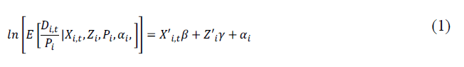
Equation (1) also has Zi variables that are time invariant and country-specific and would include a country’s socioeconomic characteristics. The αi are country-specific intercepts in a fixed effects model. Although a country’s socio-economic characteristics change over time, they are considered fixed in the time frame of this study. The time-invariant variables include life expectancy, obesity, population 65 and older, population male, medical doctors, hospital beds, diabetes, and urban population. We assume the population is constant during the sample period, so that we can move the population term to the right-hand side of the equation in Equation (2). The population variable becomes an offset in the regression. The 2020 population forecast comes from the population division. The dependent variable is countable, or Di,t=(0,1,2,3⋯) per day, which defines either a Poisson or negative binomial regression. This type of regression appears in the literature, such as Honore and Kesina, who specify this regression to model the number of doctor visits with gender and education being time-invariant after the age of 30. Meanwhile, Hausman, Hall, and Griliches model the number of patents a firm possesses based on a combination of time-varying like research and development funding and firm-specific factors such as book value and industry dummies [12].

The next manipulation is to take the exponential function of both sides of the equation and separate the time-varying and time-invariant variables by rewriting the regression as Eq. (3) by using the properties of the exponential function, where exp

We use Honore and Kesina two-step fixed-effects estimator to estimate the parameters of the model. For the first step, we estimate β either as a Poisson or negative binomial distribution and omit the time-invariant variables. This approach works because Lancaster shows the estimators for estimating β are consistent whether one includes or excludes the time-invariant variables [13]. Furthermore, the Poisson has the property where the mean equals its variance or μ=σ2. Meanwhile, the negative binomial includes a dispersion parameter, θ that allows the variance to exceed the mean, or σ2=μ+μ2/ θ. We estimate the first step using a negative binominal because the Poisson is a special case of the negative binomial. As the dispersion parameter becomes large, the variance approaches the mean in the Poisson. Both the Poisson and negative binomial distributions are common in the medical literature for cancer deaths.
The first step uses maximum likelihood to estimate β parameters, where the daily fatality from country i on day t is the dependent variable. The regression includes the number of people who have tested positive in country i on day t per million people for COVID-19. The daily cases are lagged from daily deaths because of the virus incubation period. COVID-19 requires between 2 and 14 days to grow, and an infected person is not likely to seek medical treatment until exhibiting symptoms [14]. Furthermore, a person dies, on average, 20 days after contracting COVID-19. The lag is set to 14 days, as outlined in Baud et al. [15]. At last, we apply Huber-White robust standard errors to reduce heteroscedasticity in the standard errors of the β parameter estimates, where countries induce unequal variability.
For the second step of the estimator, we have two choices. The first choice is we average the time effects over Equation (3) by rewriting as Equation (4). The Ti drops out of the equation.

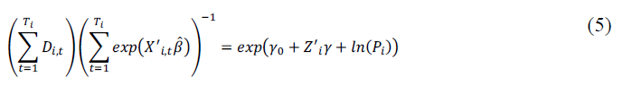
Since we have estimated the β parameters, we move the timevarying variables to the left-hand side in Equation (5). The dependent variable becomes
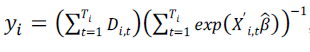
which we can view as the average deaths in country i divided by the expected deaths based only on the time-varying variables. Since we average over the time effects, a country’s specific intercept, αi, becomes a standard intercept, γ0, in Equation (5).
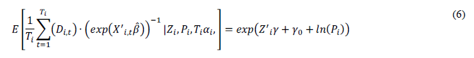
The second choice is to move the time-varying variables to the lefthand side and then average over the time effects to yield Equation 6. The dependent variable becomes
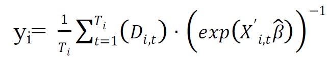
We utilize both methods in this paper.
The second step uses nonlinear least squares to estimate the γ parameters in both (5) and (6). We use the wild bootstrap to estimate the standard errors and t-statistics because the standard errors from nonlinear least squares are viewed as unreliable [16]. The wild bootstrap accounts for heteroscedasticity in the error terms because the second step transforms the panel data into cross-sectional. The number of replications is set to 200 as specified in Honore and Kesina.
Results And Discussion
In this section, we analyse how a country’s socioeconomic characteristics influence the daily fatality rate of COVID-19. We begin by plotting the data. Figure 1 plots the global daily positive cases for COVID-19 and global daily deaths in the top left and right panels. The virus continues to spread as more people test positive for the virus. The COVID-19 fatality rate reached a peak in April 2020 and dropped a little. Several observations can explain this behaviour. For example, the United States was slow to open testing centers, and the cases, in the beginning, were testing the critically ill people. South American and African countries started their epidemics at later dates, which keeps the daily fatality rate high. The bottom plots show the positive cases and deaths for the countries with the highest case counts, which are Brazil, India, Mexico, the United Kingdom, and the United States. It appears Brazil and India have attained their peaks for the number of positive test cases, while the United Kingdom and the United States are reaching new heights.

Figure 1: Daily cases and daily deaths in 2020.
We turn our attention to Figures 2 and 3, which map by country the total COVID-19 fatalities on April 30, 2020 and October 31, 2020. In April, the United States shows the highest number of deaths, followed by western European countries. Brazil, China, and Iran are slightly shaded, indicating higher fatality than the surrounding countries. In October, the deaths continue to climb with the United States still leading the world while Brazil is not far behind. The map shows new hot spots emerging in Colombia, Peru, India, Mexico, Russia, and South Africa. In sum, the maps show that movement control orders, public face mask requirements, sanitation protocols, and social distancing are not working as the virus continues to spread and claim lives.

Figure 2: Total COVID-19 deaths by country.

Figure 3: Total COVID-19 deaths by country.
We turn our attention to the descriptive statistics Table 1, panel a summarises the descriptive statistics for countries’ socioeconomic characteristics. The first three variables are time variant. Daily deaths, positive test result, and Stringency Index are bounded below by zero. The average daily global deaths over all countries in the sample time period is 31.93, while the daily average number of people testing positive is 1,414.99. The Stringency Index averages 60.02 per day as government-imposed restrictions to stop the spread of the virus. Table 1 also includes the descriptive statistics for the time-invariant variables. Life expectancy averages 73.5 years with a minimum of 54.36 years and maximum of 85.29 years. The sample has 193 countries (observations) for life expectancy. Furthermore, the per cent of the population afflicted with obesity ranges from 2.1% to 61% with a mean of 19.73% and standard deviation of 11.1%. The measure includes 191 countries. The variable with the smallest number of countries would limit a negative binomial regression to that number of countries. For example, the number of medical doctors and hospital beds reduces the number of countries to 37 and 44 countries, respectively.
| Panel A | Frequency | Time period | Min | Mean | Max | Std. dev | Observations | ||||||||
| Time-variant | |||||||||||||||
| Deaths | Daily | 1/1/2020-10/31/2020 | 0 | 31.93 | 4,928.00 | 143.75 | 50,214 | ||||||||
| Positive Cases | Daily | 1/1/2020-10/31/2020 | 0 | 1,414.99 | 234,633.00 | 7,500.22 | 50,214 | ||||||||
| Stringency index | Daily | 1/1/2020-10/31/2020 | 0 | 60.02 | 100 | 21.86 | 50,214 | ||||||||
| Time-invariant | |||||||||||||||
| Life expectancy | Annual | 2019 | 54.36 | 73.53 | 85.29 | 7.34 | 193 | ||||||||
| Obesity | Annual | 2019 | 2.1 | 19.73 | 61 | 11.1 | 191 | ||||||||
| Population 65 | Annual | 2019 | 1.09 | 8.98 | 27.58 | 6.31 | 193 | ||||||||
| Population male | Annual | 2019 | 45.46 | 50.1 | 75.5 | 3.35 | 193 | ||||||||
| Medical doctors | Annual | 2019 | 0.78 | 3.28 | 5.24 | 0.95 | 37 | ||||||||
| Hospital beds | Annual | 2019 | 0.53 | 4.3 | 12.98 | 2.63 | 44 | ||||||||
| Diabetes | Annual | 2019 | 1 | 8.33 | 30.5 | 4.73 | 210 | ||||||||
| Urban population | Annual | 2019 | 13.03 | 60.92 | 100 | 23.99 | 214 | ||||||||
| Panel B: Pearson correlation | |||||||||||||||
| Time invariant | (1) | (2) | (3) | (4) | (5) | (6) | (7) | (8) | |||||||
| Life expectancy | 1 | ||||||||||||||
| Obesity | 0.51 | 1 | |||||||||||||
| Population 65 | 0.74 | 0.3 | 1 | ||||||||||||
| Population male | 0.04 | 0.14 | -0.34 | 1 | |||||||||||
| Medical doctors | 0.29 | 0.21 | 0.56 | -0.17 | 1 | ||||||||||
| Hospital beds | 0.17 | -0.33 | 0.53 | -0.31 | 0.13 | 1 | |||||||||
| Diabetes | 0.21 | 0.49 | -0.07 | 0.29 | -0.35 | -0.23 | 1 | ||||||||
| Urban population | 0.61 | 0.48 | 0.48 | 0.15 | 0.09 | 0.03 | 0.02 | 1 | |||||||
Table 1: Descriptive statistics.
Panel A summarises the descriptive statistics of the data used in this study. Panel B shows the Pearson correlation between the socioeconomic variables.
Table 1, panel B shows the Pearson correlations for countries’ socioeconomic characteristics. For example, diabetes measure positively correlates with life expectancy (0.21) obesity (0.49) and males (0.29) and negatively correlates with the number of doctors (-0.35) and hospital beds (-0.23). Furthermore, the obesity measure positively correlates with the population of 65 and older (0.30) and urban population (0.48) and negatively correlates to the number of hospital beds (-0.33).
We apply the two-step fixed-effects estimator on four models. For the first stage, the observations range between 8,852 and 36,719 with the smallest number of countries (36) in model 1 and the highest number of countries (171) in models 3 and 4. Furthermore, the theta ranges between 0.1644 and 0.2591 and indicates the variance is overdispersed, and the negative binomial is the appropriate choice.
Table 2 shows the parameter estimates for the first step in the twostep fixed-effects estimator for the time-varying variables. The number of people testing positive for COVID-19 per one million people is positive and statistically significant in all models. This should not be surprising because as the number of people testing positive for COVID-19 rises, we would expect more deaths. Furthermore, the quadratic trend is statistically significant in all models, and the daily fatality rate exhibits an upside-down U-shape. As predicted, a country experiences a rise in COVID-19 deaths, attains a peak, and the deaths begin falling for the first wave. We solve for the number of days when a country reaches its peak after registering their first positive test case. Consequently, a country reaches its peak in COVID-19 deaths from 258.1 and 387.7 days after having its first positive test case. At last, the stringency index is positive and statistically significant for all models. This result is not unusual because policymakers react to deaths. As deaths from COVID-19 rise and hospitals are filled to overcapacity, governments are likely to impose stringent measures over their constituents to contain and stop the spread of the virus.
| Model 1 | Model 2 | Model 3 | Model 4 | |
| Countries | 36 | 43 | 163 | 163 |
| Observations | 8,852 | 10,476 | 36,719 | 36,719 |
| Theta | 0.2476 | 0.2591 | 0.1644 | 0.1644 |
| First step | ||||
| Intercept (β0) | -3.4513** (-15.9791) | -3.5109** (-17.6346) | -2.1128** (-19.5868) | -2.1128** (-19.5868) |
| Cases | 0.0134** (12.8946) | 0.0107** (12.4737) | 0.0232** (29.4511) | 0.0232** (29.4511) |
| Trend | 0.0124** (12.8946) | 0.0120** (12.4737) | 0.0107** (29.4511) | 0.0107** (29.4511) |
| Trend 2 | -1.92E-05** (-3.0818) | -1.54E-05** (-2.7861) | -2.08E-05** (-4.4981) | -2.08E-05** (-4.4981) |
| Stringency index | 0.0872** (38.3714) | 0.0879** (40.2001) | 0.0511** (47.9302) | 0.0511** (47.9302) |
| Second step | ||||
| Intercept (γ0) | 29.8734 (0.1632) | 33.4783** (12.1926) | -3.5477** (-16.2820) | -3.5205** (-16.0125) |
| Life expectancy | -0.0867** (-4.9902) | -0.0582** (-2.2433) | 0.1608** (49.0709) | 0.1432** (48.3747) |
| Obesity | 0.0505** (8.5062) | 0.0316** (3.0061) | 0.0362** (60.1559) | 0.0320** (59.9114) |
| Population 65 | 0.1539** (5.5494) | 0.1096** (7.9644) | -0.3902** (-88.8506) | -0.4047** (-86.5519) |
| Male population | -0.5872 (1.2301) | -0.6959** (-10.6431) | -0.2081** (-51.4511) | -0.1856** (-48.2244) |
| Medical doctors | -1.0509** (-2.5711) | |||
| Hospital beds | -0.5474** (-13.3906) | |||
| Diabetes | 0.0189** (16.7445) | |||
| Urban population | 0.0089** (23.1435) | |||
Table 2: Parameter estimates of the two-step fixed-effects estimator.
The table summarises the parameter estimates and z-stats (t-stats) from Honore and Kesina two-step fixed-effects estimator show below.

The first step estimates the β parameters using a negative binomial regression that excludes the time-invariant variables. The dependent variable is daily deaths, Di,t, in the country i on day t. The explanatory variables (Xi,t) include positive test cases per million lagged 14 days, a quadratic trend, and the stringency index. Huber-White robust standard errors reduce the heteroscedasticity from each country’s variation on the standard error. The table includes the z-statistics in parentheses. The second step estimates the γ parameters for a country’s socioeconomic characteristics (Zi) using nonlinear least squares. The dependent variable is

A wild bootstrap with 200 replications estimates the standard errors and t-statistics. The ∗∗, and ∗ denote significance at the 1%, and 5% levels, respectively.
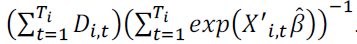
The second step in the fixed-effects estimator is to estimate the parameters for the time-invariant variables. The second step reduces the number of observations to the number of countries because we average over the time effects. Model 1 has the fewest observations, which are 36 countries, while models 3 and 4 have the most with 162 countries. We calculate the new dependent variable as
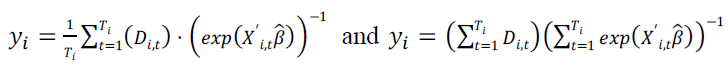
Both variables are positively correlated, which range between 0.79 and 0.86. Both measures have a lower bound of zero, but the first dependent variable consistently has a higher upper bound than the second dependent variable. However, the second dependent variable leads to more statistically significant variables for the second step, whose parameter estimates are reported in Table 2.
The results from the second step show the life expectancy is negative and statistically significant in models 1 and 2, and positive and statistically significant in models 3 and 4. We would expect life expectancy to be negative because people living in countries with better health care and sanitation live longer on average than countries with lower life expectancies.
Two factors could cause parameter estimates to switch signs even though they remain statistically significant. First, endogeneity problem could cause parameter estimates to switch signs. The endogeneity could result from a missing variable. One correction method is to increase the number of observations. Models 3 and 4 have at least four times the number of countries than models 1 and 2. Furthermore,multi-collinearity could cause signs to change on parameter estimates. Table 3 shows the results from the variance inflation factors. The highest value is 3.3177, which suggests a low level of multicollinearity exists between the variables.
|
|
Model 1 |
Model 2 |
Model 3 |
Model 4 |
|
Life expectancy |
1.8551 |
2.1337 |
3.2882 |
3.3027 |
|
Obesity |
1.55 |
1.9602 |
1.5133 |
1.504 |
|
Population 65 |
2.7847 |
2.4566 |
3.3177 |
3.2575 |
|
Male population |
1.9441 |
2.2447 |
1.4773 |
1.5365 |
|
Medical doctors |
1.6039 |
|
|
|
|
Hospital beds |
|
1.9577 |
|
|
|
Current smokers |
|
|
|
|
|
Diabetes |
|
|
1.3636 |
|
|
Unemployment |
|
|
|
|
|
Urban population |
|
|
|
1.8809 |
Table 3: Variance inflation factor.
Table contains the Variance Inflation Factors (VIF) for each regression in Table 2. The VIF is estimated for the variables in the second stage of estimation with the dependent variable
The VIF does not depend on the regression’s functional form.
The next variable is the per cent of the population who are obese. Obesity is positive and statistically significant in all models. The parameter estimates vary over a small range, which indicates the parameter estimates are robust as the number of counties changes in the sample. Furthermore, the endogeneity problem may not be severe. Furthermore, we would expect the parameter estimate to be positive because obesity is associated with a host of problems called metabolic syndrome, which includes heart disease, high blood pressure, stroke, and type 2 diabetes. People afflicted with these conditions are susceptible to complications from COVID-19. In addition, model 3 has the per cent of the population with diabetes. It is also positive and statistically significant. In sum, both obesity and diabetes raise the daily COVID-19 fatality rate.
The variable, population 65 and older, shows mixed results. Although all parameter estimates are statistically significant, models 1 and 2 are positive and statistically significant with the correct sign, while models 3 and 4 are negative and statistically significant. As already discussed, multicollinearity could cause these problems since the VIF in Table 3 rises for the population age 65 and older. As Table 1 shows, many of a country’s socioeconomic characteristics are highly correlated, such as life expectancy, age 65 and older, obesity, and diabetes. In addition, the elderly in retirement homes are particularly vulnerable because of staff shortages from sick staff and restrictions that prevent family visits and monitoring, which could increase the fatality rate from COVID-19 [17].
The variable, percentage of males, is not significant in model 1 but significant in the other models. However, models 2, 3, and 4 have the wrong sign. This odd result could originate from most countries having a population of 50/50 males and females with little variability between countries.
The next variables measure the level of medical resources a country possesses. Both medical doctors per 1,000 people and hospital beds per 1,000 people are negative and statistically significant in models 1 and 2. Even though countries can expand their hospital bed capacity by organizing and building temporary intensive care units to care for COVID-19 patients, hospital beds in this model indicate a country’s medical resource level. As a country starts with more doctors and hospital beds before the pandemic can expand medical services as needed during a pandemic. The results corroborate Stojkoski, Utkovski, Jolakoski, Tevdovski and Kocarev and Sussman that the medical sector must possess resources to combat the COVID-19 pandemic [18]. The results also confirm that developing countries may exhibit higher daily death rates from COVID-19 because of the lack of medical resources to treat the medical complications of COVID-19. Consequently, social distancing and movement control orders could slow the number of people becoming infected with COVID-19 and help a country with limited medical resources to battle an epidemic [19]. The last variable, urban population, is positive and statistically significant in model 4. We expect this result because COVID-19 would spread faster in urban areas with dense populations. Consequently, social distancing, school and work closures, and stay at home orders could slow the spread of the virus as people minimize their contact with other people.
Conclusion
This paper has examined the relationship between a country’s socioeconomic characteristics and their influence on the daily COVID-19 fatality rate. The results show the two-step fixed-effects estimator can estimate the time-invariant parameters. As we would expect, a country with a higher number of medical doctors and hospital beds in a country reduce the complications of COVID-19 by lowering the fatality rate. Meanwhile, a country with more obese, diabetics, elderly, and urban population raise the COVID-19 fatality rate while a higher life expectancy lowers it. At last, the results further indicate that the daily fatality rate from COVID-19 is positively related to the number of people testing positive for COVID-19 and the stringency index. The unusual result with the stringency index may stem from governments’ reaction to the pandemic as they impose harsher orders to contain and stop the spread of the virus as the COVID-19 deaths rise in their countries.
This paper provides four public policy recommendations. First, governments should encourage universities and health ministries to establish new medical schools and expand the capacity of existing medical schools to raise the number of doctors and expand hospital capacities with more beds. Countries endowed with medical resources have higher life expectancies. Second, the elderly have a higher risk of dying, so governments should encourage the elderly to stay at home during outbreaks and ensure they have access to health care. Government inspectors should check and monitor the elderly in longterm care facilities to ensure proper staffing levels and good treatment of the elderly. Third, governments should encourage their citizens to maintain healthy body weight since obesity leads to a host of medical problems, such as type 2 diabetes. Finally, urban populations are more susceptible to COVID-19, and governments must react quickly to contain and stop the spread of viruses.
Acknowledgements
No external help was used in this study.
Funding Sources
This research did not receive any specific grant from funding agencies in the public, commercial, or not-for-profit sectors.
Ethical Approval
This study is exempt from IRB review.
Funding
No funding was utilized for this research.
Competing Interests
The authors report no conflicts of interest.
References
- Guan WJ, Ni ZY, Hu Y, Liang WH, Ou CQ, et al. (2020) Clinical characteristics of coronavirus disease 2019 in China. N Engl J Med 382: 1708-1720.
[Crossref] [Google Scholar] [PubMed]
- Remuzzi A, Remuzzi G (2020) COVID-19 and Italy: What next? Lancet 395: 1225–1228.
[Crossref] [Google Scholar] [PubMed]
- Wu Z, McGoogan JM (2020) Characteristics of and important lessons from the Coronavirus disease 2019 (COVID-19) outbreak in China: Summary of a report of 72314 cases from the Chinese center for disease control and prevention. JAMA 323: 1239-1242.
[Crossref] [Google Scholar] [PubMed]
- Zheng YY, Ma YT, Zhang JY, Xie X (2020) COVID-19 and the cardiovascular system. Nat Rev Cardiol 17: 259-260.
[Crossref] [Google Scholar] [PubMed]
- Mikhael EM, Al-Jumaili AA (2020) Can developing countries alone face Coronavirus? An Iraqi situation. Public Health Pract 1: 100004.
[Crossref] [Google Scholar] [PubMed]
- Honore BE, Kesina M (2017) Estimation of some nonlinear panel data models with both time-varying and time-invariant explanatory variables. J Bus Econ Stat 35: 543-558.
[Crossref] [Google Scholar] [PubMed]
- Hawkins RB, Charles E, Mehaffey J (2020) Socio-economic status and COVID-19 related cases and fatalities. Public Health 189: 129-134.
[Crossref] [Google Scholar] [PubMed]
- Mukherji N (2020) The social and economic factors underlying the impact of COVID-19 cases and deaths in US counties. MedRxiv.
- Sa F (2020) Socioeconomic determinants of COVID-19 infections and mortality: Evidence from England and Wales. Covid Econ 47-58.
- Cao Y, Hiyoshi A, Montgomery S (2020) COVID-19 case-fatality rate and demographic and socioeconomic influencers: Worldwide spatial regression analysis based on country-level data. BMJ Open 10: e043560.
[Crossref] [Google Scholar] [PubMed]
- Stojkoski V, Utkovski Z, Jolakoski P, Tevdovski D, Kocarev L (2020) The socio-economic determinants of the Coronavirus disease (COVID-19) pandemic. MedRxiv.
- Hausman JA, Hall BH, Griliches Z (1984) Econometric Models for count data with an application to the patents-R and D relationship. 52: 909–938.
- Lancaster T (2002) Orthogonal parameters and panel data. Rev Econ Stud 69: 647-666.
- Cascella M, Rajnik M, Aleem A, Dulebohn SC, di Napoli R (2023) Features, evaluation, and treatment of Coronavirus (COVID-19). StatPearls Publishing, Treasure Island (FL).
[Google Scholar] [PubMed]
- Baud D, Qi X, Nielsen-Saines K, Musso D, Pomar L, et al. (2020) Real estimates of mortality following COVID-19 infection. Lancet Infect Dis 20: 773.
[Crossref] [Google Scholar] [PubMed]
- Tellinghuisen J (2018) Can you trust the parametric standard errors in nonlinear least squares? Yes, with provisos. Biochim Biophys Acta Gen Subj 1862: 886-894.
[Crossref] [Google Scholar] [PubMed]
- Gardner W, States D, Bagley N (2020) The Coronavirus and the risks to the elderly in long-term care. J Aging Soc Policy 32: 310-315.
[Crossref] [Google Scholar] [PubMed]
- Sussman N (2020) Time for bed(s): Hospital capacity and mortality from COVID-19. COVID Econ 11: 116-131.
- Ferguson NM, Laydon D, Nedjati-Gilani G, Imai N, Ainslie K, et al. (2020) Impact of Non-Pharmaceutical Interventions (NPIs) to reduce COVID-19 mortality and healthcare demand. London: Imperial College London. 1-20.
Citation: Szulczyk KR, Cheema MA, Ziaei SM (2025) COVID-19: The Impact of Socioeconomic Characteristics on the Fatality Rate. J Community Med Health Educ 15: 912.
Copyright: © 2025 Szulczyk KR, et al. This is an open-access article distributed under the terms of the Creative Commons Attribution License, which permits unrestricted use, distribution and reproduction in any medium, provided the original author and source are credited.
Select your language of interest to view the total content in your interested language
Share This Article
Recommended Journals
Open Access Journals
Article Usage
- Total views: 348
- [From(publication date): 0-0 - Dec 10, 2025]
- Breakdown by view type
- HTML page views: 268
- PDF downloads: 80