Identifying Long-Memory Trends in Pre-Seismic MHz Disturbances through Support Vector Machines
Received: 30-Dec-2014 / Accepted Date: 18-Feb-2015 / Published Date: 28-Feb-2015 DOI: 10.4172/2157-7617.1000263
Abstract
In this paper, a novel algorithm is introduced for the analysis of long-memory patterns hidden in electromagnetic (EM) readings prior to earthquakes. The algorithm builds upon previous work on long-memory detection in EM measurements by fusing Support Vector Machine (SVM) classifiers with well-deployed power law fit tests and Rescaled-Range (R/S) time-series variability methods. To apply the algorithm, fractal power law in the wavelet domain is assessed so as to identify fractional Brownian motion (fBm) segments of continuously monitored pre-earthquake EM activity. The selected segments are then further processed through R/S Analysis in order to further refine the detection of prominent fBm behaviour. The combined output of the two methods is used to train a SVM classifier which is subsequently employed to verify similar fBm states in existing EM data and to allow for rapid fBm detection in large data sequences of unprocessed or newly incoming EM readings. The SVM classifier is added in a modular fashion, on top of pre-earthquake monitoring algorithms, and can be trained with a small fraction of a huge available dataset of EM readings. Three earthquake events in Greece, corresponding to different time occurrences and geographic locations, were investigated. For each of the three earthquakes, data collected by a nearby EM measurement station one month prior to the peak event were analysed by the proposed method. The results yielded an overall accuracy rate of at least 90% for the detection of specific, prominent fBm segments despite the fact that the fBm profile in the three investigated earthquake sequences was very different.
Keywords: Seismic effects; Spearman correlation coefficient; Support vector machine
8832Introduction
Several electromagnetic (EM) phenomena have been declared as precursory, viz. observed prior to earthquakes. The stated precursory EM frequency range includes ultra-low frequencies (ULF) from 0.001 to 1 Hz [1-7], low frequencies (LF) between 1 and 10 kHz [6,8-13], high frequencies (HF) between 40 and 60 MHz [6,8,14-17] and very high frequencies (VHF) up to 300 MHz [18]. A principal method for identifying pre-earthquake precursors is the direct observation of EM emissions from the lithosphere [5]. A significant alternative is the indirect detection of seismic effects that take place in a form of propagation anomaly due to existing transmitter signals [5]. The underlying idea is that the EM disturbances emerge from the hypocentre of earthquakes due to the tectonic effects that accompany their preparation phase [5]. This renders additional indirect seismic effects in the form of disturbances propagation generated by pre-existing transmitter signals in the atmosphere and ionosphere [5]. According to some investigators, the pre-existing transmitters are inside the earth's crust [6]. According to several publications [10,11,19], the transmitters are the dynamically unstable multi-cracks that are continuously generated and moved during the earthquake preparation process. It is this transmission that causes the rupture of inter-atomic (ionic) bonds on the surfaces of new micro-cracks and evokes intense surface-charge separation, making micro-cracks effective electric dipoles and efficient electromagnetic emitters prior to earthquakes. Note that these failure-induced crackbased electromagnetic disturbances are observed not only in nature but also under controlled experimental conditions [9-11,20]. The variety, however, of the several electromagnetic precursors and the wide ranges of values of time delay between events and observed earthquakes [11,21] complicates the analysis and limits significantly the possibilities of prediction. Adding to this complexity, is the multitude of methods employed to detect the EM anomalies and the different viewpoints from which the problem is seen.
A framework shared by a number of analysis methods is founded on the long-memory trends of data sequences and specifically on evidence of fBm behavior [3-5,8-11,14]. Examples of methods on long-memory analysis of time series are the power law fit test in a transform domain [3,4,8-10,14,17,22], the Rescaled Range (R/S) Analysis [10,16,23] and the Detrended Fluctuation Analysis method (DFA) [10,16], among others. The outputs of these methods are not always in agreement, partly due to the difficulty of the problem at hand. Therefore, the task of combining two or more of the long-memory analysis methods to achieve better results arises naturally. In this paper, we attempt to combine the power law fit test in the wavelet domain, named hereafter power-law wavelet method, with the R/S method in order to improve the detection capability of a continuous EM radiation monitoring system.
Continuous monitoring of pre-earthquake EM emissions involves large data processing and real-time results delivery. This brings forth the need for a method able to handle large data sets and perform fast computations that will work in conjunction with existing, state-ofthe- art long-memory analysis techniques. To this end, the feasibility of a supervised classification algorithm is explored, namely the SVM classifier [24], known for its simple theoretical foundation and powerful modeling capabilities. To our knowledge, this is the first time the SVM is used for the detection of precursory signs in pre-seismic EM radiation, although it has been proposed as a warning system for standard (ground vibration) seismic signals [25]. The SVM classifier’s role is twofold. First, it is used to verify the findings of the two long-memory analysis methods, i.e. the joint findings of the power law wavelet and R/S methods. Second, in a scenario where continuous monitoring of EM signals is required, the SVM can classify recorded EM signal segments into their prominent fBm parts and those not exhibiting such behavior much faster than the two long-memory analysis methods combined. In addition, it is of importance to determine if EM signals, categorized as prominent fBm or not by standard long-memory analysis methods, are also clearly separable in a high dimensional feature space, created naturally by the SVM methodology.
The whole algorithm was tested on three significant earthquakes (i.e. larger than ML=5) which occurred at different locations and times in Greece. In general, EM radiation data at 3 kHz, 10 kHz, 41 MHz and 46 MHz frequencies are continuously collected by a telemetric network which operates in Greece almost uninterruptedly [26]. In each of these signals, recorded by a station located on a 50 km radius around the corresponding epicenter and up to one month prior to the ensuing earthquake, a combination of the power law wavelet and R/S methods was applied on the EM time series in order to discover prominent fBm patterns. The output of the long-memory analysis methods was used to label the EM data as prominent fBm and not prominent fBm or nonfBm in order to facilitate the design of a two-class SVM classifier.
The present paper reports a new method on the detection of prominent fBm state behavior of EM measurements. In the first step of the proposed method, the two main long-memory analytic techniques are described, namely the power-law wavelet method and the R/S analysis. A twofold scheme is presented, as an intersection between the above two long-memory analysis techniques, in order to detect specific, prominent, fBm signatures. In the second step, the combined scheme is used for training a SVM classifier. The SVM training and classification process is described, along with the selected signal features that are used to reduce the amount of data sent to the classifier. Next, the predictability and reproducibility of the SVM classifier in terms of discriminating between prominent fBm and not prominent fBm or non-fBm classes in a high dimensional feature space are analyzed. The performance of the SVM classification stage is highlighted and the close agreement with the long-memory analysis methods is verified. Concluding remarks are given at the end
Methods
The methods developed in this work are generally divided into the long-memory analysis methods and the classification methods. Initially, a combination of two long-memory analysis methods is employed on the EM data to detect anomalies prior to significant earthquake events. These two methods, namely the power-law wavelet and the R/S analysis methods, are described in the next subsections. The output of the R/S method is expressed in terms of the Hurst exponent (H), a mathematical quantity which can detect long-range dependencies in time-series [27,28].
After the two-method analysis has labeled the significant versus the insignificant signal segments, a SVM classifier is trained on a small part of the labelled data and tested on the remaining or newly incoming data. It is desirable for the SVM to quickly compute the training parameters and to be able to classify new data rapidly. Signal features are thus derived that reduce the data dimensions and, at the same time, attempt to capture the information that is critical for classification. The general SVM framework is described in the next subsections, along with an efficient features selection scheme for data reduction.
Power-law Wavelet Fractal Analysis Method
During the complex process of earthquake preparation, linkages between space and time produce characteristic fractal structures [3,4,6,10,16,18]. It is expected that these fractal structures affect signals rooted in the earthquake generation process. The power spectrum density (PSD), is probably the most commonly used technique to provide useful information about the inherent memory of the system [10]. Although the power spectrum is only the lowest order statistical measure of the deviations of the random density field from homogeneity, it directly reflects the physical scales of the processes that affect structure formation [10]. If the recorded time-series,
 , is a temporal fractal, then a power-law spectrum is expected, i.e., S(f)=α·f -b, where f is the frequency of the transform. In a log(S( f ))− log( f ) representation, the power spectrum is a straight line, with linear spectral slopeb. The spectral amplificationα quantifies the power of the spectral components following the power spectral density law. The spectral scaling exponentbis a measure of the strength of time correlations. In the case of 1<b<3, the time series profile is considered to be a temporal fractal associated with fBm. The goodness of the power-law fit to a time-series is represented by the Spearman’s linear correlation coefficient r[10]. Attention is paid to whether distinct changes in the scaling exponent emerge before or during any detected bursts.
For the investigation the following steps were followed:
(i) The MHz EM signals were divided in segments (windows) of 1024 samples. These segmentations were expected to reveal the fractal characteristics of the signals [10,16,17].
(ii) In each segment the PSD of the signal was calculated. For the PSD calculation, the CWT using the Morlet wavelet was employed.
(iii) In each segment the existence of a power-law  was investigated. In the PSD calculation, the employed frequency f was the central frequency of the Fourier transform of the Morlet scale.
(iv) The least square method was applied to the linear representation. Successive representations were considered those that exhibited squares of the Spearman's correlation coefficient above 0.95, i.e., 95% confidence interval with
Estimation of Hurst exponent through R/S analysis
Hurst exponent is a mathematical quantity which can detect longrange dependencies in time-series [27,28]. It can estimate the temporal smoothness of time-series and can search if the related phenomenon is a temporal fractal [29]. Hurst exponent was conceptualized for hydrology [27,28]. It has been employed however in other research topics as well, for example, traffic traces [30], plasma turbulence [31], ULF geomagnetic fields [4,5], climatic dynamics [32], pre-epileptic seizures [29], astronomy and astrophysics [33] and economy [34]. H-values between 0.5<H<1 manifest long-term positive autocorrelation in time-series. This means that a high present value will be, possibly, followed by a high future value and this tendency will last for long future time-periods (persistency) [8,14,35,36]. H values between 0<H<0.5 indicate time-series with long-term switching between high and low values. Namely, a high present value will be, possibly, followed by a low future value, whereas the next future value will be high and this switching will last long, into future (anti-persistency) [8,14,35,36]. H=0.5 implies completely uncorrelated time-series.
Hurst exponents were estimated through the method of Rescaled Range (R/S) [29] or as frequently referred, R/S analysis. The R/S analysis was introduced by Hurst [27] and attempts to find patterns that might repeat in the future. The method employs two variables, the range, R, and the standard deviation, S, of the data. According to the R/S method, a natural record in time, is transformed into a new variable
 in a certain time period n (n =1,2,...,N) from the average,
  , over a period of N time units [27]. y(n, N) is called accumulated departure of the natural record in time [27]. The transformation follows the formula:
 (1)
(1)
The rescaled range is calculated from (2) [23,27,29]:
 (2)
(2)
The range R(n) in (2) is defined as the distance between the minimum and maximum value of y(n, N) by
 (3)
(3)
The standard deviation S(n) in (2) is calculated by
 (4)
(4)
R/S is expected to show a power-law dependence on the bin size n
 (5)
(5)
where H is the Hurst exponent and C is a proportionality constant.
The log transformation of the last equation is a linear relation
 (6)
(6)
from which, exponent H can be estimated as the slope of the best line fit.
SVM classification
The EM data processed by the long-memory analysis methods are labeled as prominent fBm or not in terms of the presence, or not, of successive (r2>0.95) fractal fBm structure and a Hurst exponent above a certain threshold value. Two-class segmentation thus arises, which can be elegantly handled by a supervised classifier. Among the several classifiers, the SVM classifier is selected for its simplicity and the fact that no prior information or assumptions on the treated EM data is required. In its most basic form, SVM attempts to separate already labelled data via a hyperplane into two regions (classes) such that the gap between them is maximized, i.e., the point of class A closest to the hyperplane and the point of class B closest to the hyperplane are as far apart as possible. The data can also be mapped onto another, higher dimensional, space via a kernel function in case they are not linearly separable in the existing space.
The EM segments are typically of high length (e.g. 1024 samples each), which means that the SVM will have to process very long vectors during its training phase, i.e., during the derivation of the separating hyperplane. For this reason, it is wise to reduce the segments length by deriving features of much shorter length but of high information content. Typical features are found in a transform domain such as the Discrete Wavelet Transform (DWT). The DWT, used as a filterbank, is critically sampled meaning that its output is of the same length as its input signal and so there is no redundancy. It produces subband signals with adjustable frequency and time resolution. The actual filterbank scheme can be collapsed into two filtering operations [37], i.e.,
 (7)
(7)
 (8)
(8)
where α(i)[n] and d(i)[n] are the nth coefficients of the approximation and detail vector, respectively, at level i. They are the outputs of the lowpass wavelet filter g and highpass wavelet filter h after downsampling by a factor of two. The addition of the approximation and detail signals at level i produces the approximation signal at level i-1. Starting with the 0th level approximation signal as the original signal, a tree-like structure of the DWT filterbank is evident. The frequency bands of α(i) and d(i) span the lower half and upper half, respectively, of the frequency band of α(i-1) . Notice that as the frequency bandwidth is reduced in each level, we can downsample the signal thus reducing the number of samples. In contrast, the CWT does not employ downsampling after each scale is applied and the redundancy is higher.
For our scheme we select a three-level tree structure for the DWT with the Haar wavelet as its basis function which is preferred for its great time localization capability. The jth EM data segment enters the DWT filterbank to produce the approximation signal vector at level 3, . Based on the filterbank description above, the vectors correspond to a frequency band that spans the lower 1/8 of the EM spectrum. This is desirable since we are mostly interested in the low frequency content of the EM data sequence. Higher frequency information is incorporated with the use of statistical descriptors. More specifically, for each of the six sub-band signals
  and we derive the standard deviation as
  and the standard deviation of the correlation function as
  .Each signal is further normalized to zero mean and standard deviation equal to one by subtracting the mean from each and dividing by its standard deviation. This last operation maps helps to improve the classifier performance. The final feature vector of the jth EM segment can be written as
 (9)
(9)
The feature vectors x are built to be used during the training phase of the SVM classifier as well as during the testing phase. The criteria for separating these features into classes are analyzed next.
Class separation via long-memory analysis methods
The SVM classification algorithm, being a supervised learning method, requires class-labelling of the segments or vectors that are used for initially training the classifier. Our goal is to find a reliable criterion to label the EM segments that are afterwards used for training the SVM classifier. For our scenario we need two classes. Class I (prominent successive fBm class) consists of EM segments that are deemed as significant or of some earthquake precursory value. Class II (not prominent fBm or non-fBm class) consists of EM segments that are deemed as insignificant or of no earthquake precursory value. Apparently, Class II EM segments are the complement of Class I segments. The two long-memory analysis methods described previously, i.e. the powerlaw wavelet and R/S methods, are combined here in terms of their common output, the Hurst exponent, in order to establish a criterion for separating the EM segments into significant or insignificant entities.
We first employ the powerlaw wavelet method as it is the standard method for detecting temporal fractals in data. For all the training EM segments processed, we search for the particular segments that show strong fractal behavior, given by spearman’s correlation coefficient r with values r2>0.95. A second screening is applied on the segments with r2>0.95 to find the ones with b exponent in the range 1<b<3 which indicates fBm behavior. The R/S method is then applied on the segments in order to further refine the fBm tracking process and the Hurst exponents are computed. As it is shown later in the results, the Hurst exponents of the segments with r2>0.95 and 1<b<3 (successive fBm segments) are generally higher as compared to the Hurst exponents of the segments with r2>0.95 and 1<b<3 (non-successive fBm segments) or with  (non-fBm segments). Under this observation, a minimum threshold operator can be applied on all the EM segments as a multiple of the mean Hurst exponent value M of the total of non-fBm and non- successive fBm segments in order to isolate the successive fractal fBm segments with high Hurst exponents. Hence, we define:
Class I segments as the successive fractal fBm segments (r2>0.95 and 1<b<3 ) with H above the threshold.
Class II segments as the successive fBm segments with H below the threshold and also all the remaining (cases of non-successive fBm segments viz., with r2>0.95 and 1<b<3 and cases of non-fbm segments, viz. with .
The aforementioned segments, along with their class annotation, are used as training data for the SVM classifier in order to derive its training parameters. The overall algorithmic procedure is presented in the form of a flowchart in Figure 1.
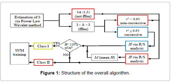
Figure 1: Structure of the overall algorithm.
In the testing phase, the SVM classifies the testing data according to the stored training parameters. For a specific kernel function  and mapping f(·) of the feature vector x to a higher dimensional feature space, the decision process for classifying the testing data into Class I or Class II is given by
  with sgn(·) the sign function and w, b part of the training parameters. The important point here is that once the training of the SVM is complete, i.e. the training parameters are derived, the decision process is very fast computationally. It is given by the sign of the inner product of two vectors, w and φ (x) , after having been added to the constant b. In comparison, the original method of identifying Class I segments by first applying the powerlaw wavelet method and then the R/S method incurs a much higher computational cost.
Implementation and Results
The algorithm described above is implemented for the scenario of EM data monitoring, prior to earthquakes in Greece. By utilizing an extensive network of EM monitoring stations [26], we explore three major earthquakes (ML>5) in a time period starting one month before each earthquake occurrence. Each EM data sequence consists of emission readings corresponding to 41 MHz radiation with a sampling frequency of 1 Hz. This amounts to a sequence length of approximately 2.6x10⁶ samples for a 30-day recording. The EM segment size is set to 1024 samples. In our implemented scenario, we assume that we are continuously searching for anomalies in the EM readings without knowing the time of occurrence of the earthquake peak event. Fractal analysis through the described algorithms is done on a regular basis, e.g., at the end of each monitored day. Real time processing is more difficult, as long-memory analysis methods operate on successive, fixed length segments (e.g. 1024 samples), advancing one sample ahead each time i.e. the sliding window step is one sample. With these parameters, the analysis captures very fine EM variations in time at the expense of high computational cost as any given fractal analysis window almost completely overlaps the preceding one. Given the same window length and step size, and once the SVM training is complete, the SVM classification task can be performed much more rapidly and real time processing is less computationally demanding.
The three EM recordings, corresponding to the three different earthquakes under investigation, are shown in Figure 2. The first investigated recording corresponds to a 30-day pre-seismic EM activity before the earthquake of magnitude ML= 5.8 occurring south of Crete island (34.35 °N 25.40 °E) on 01/07/2009 (or JD 182 2009 in Julian’s calendar format) at the depth of 30 km, captured by a station in Neapoli. During this 30-day activity, two additional earthquakes occurred prior to the main ML=5.8 event in a 50 km radius near the Neapoli station. The first additional earthquake ML=5.0 occurred on 26/6/2009 (JD 177, 2009) at 36.53 °N 25.49 °E at the depth of 28 km. The other additional earthquake ML=5.4 occurred on 19/6/2009 (JD 170, 2009) at 36.46 °N 28.31 °E at the depth of 42 km. The second investigated recording corresponds to a 30-day pre-seismic EM activity before the earthquake of magnitude ML=6.2 occurring west of Crete island (35.50 °N 23.28 °E) on 12/10/2013 (or JD 285 2013 in Julian’s calendar format) the depth of 65 km, captured by a station in Neapoli. The third investigated recording corresponds to a 30-day pre-seismic EM activity before the earthquake of magnitude ML=6.3 occurring north of Limnos island (40.29 °N 25.40 °E) on 24/05/2014 (or JD 144 2014 in Julian’s calendar format) at the depth of 30 km, captured by a station in Mytilene island.
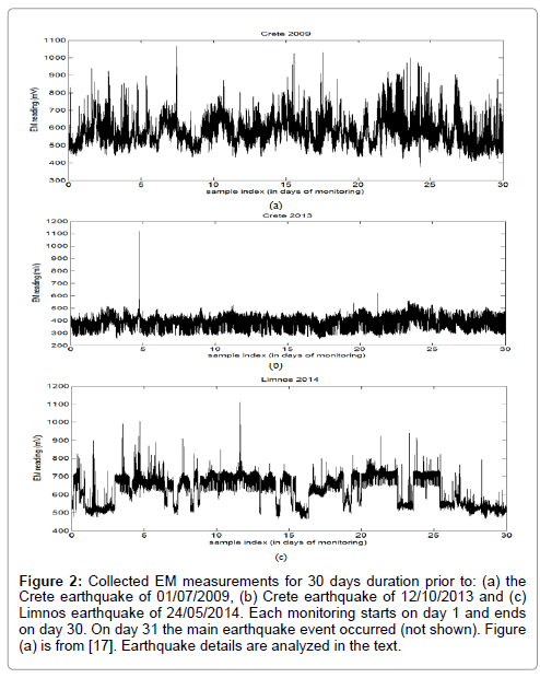
Figure 2: Collected EM measurements for 30 days duration prior to: (a) the Crete earthquake of 01/07/2009, (b) Crete earthquake of 12/10/2013 and (c) Limnos earthquake of 24/05/2014. Each monitoring starts on day 1 and ends on day 30. On day 31 the main earthquake event occurred (not shown). Figure (a) is from [17]. Earthquake details are analyzed in the text.
Figure 3 presents the results from the powerlaw wavelet method for the sequences of Figure 2 leading to (a) the Crete earthquake of 01/07/2009, (b) the Crete earthquake of 12/10/2013 and (c) the Limnos earthquake of 24/05/2014. Figure 3(a) analyzes the same data as in [17] but with different analysis parameters. The blue points represent the case of successive fBm segments, i.e., the case with r2>0.95 and 1<b<3 . The red points represent the case of non-successive fBm or non-fBm segments, i.e., the case with r2>0.95 and 1<b<3 , or with
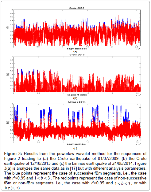
Figure 3: Results from the powerlaw wavelet method for the sequences of Figure 2 leading to (a) the Crete earthquake of 01/07/2009, (b) the Crete earthquake of 12/10/2013 and (c) the Limnos earthquake of 24/05/2014. Figure 3(a) is analyzes the same data as in [17] but with different analysis parameters. The blue points represent the case of successive fBm segments, i.e., the case with r2>0.95 and 1<b<3 . The red points represent the case of non-successive fBm or non-fBm segments, i.e., the case with r2>0.95 and 1<b<3 , or with b€(1, 3) .
It can be observed that all subplots present several segments with the square of the Spearman correlation coefficient above the critical value of 0.95, i.e., the fit to the power-law was excellent. This is a strong indicator of the fractal character of the underlying processes and structures [10,11]. It is important that the successive power-law beta-values were between 1 and 3. Power-law b-exponent values in the range 1.5<b<2 indicate well-established fractal fBm anti-persistency and values above 2 (b>2) fBm persistency. The latter implies that the corresponding fluctuations are positively correlated. This suggests that the underlying dynamics are governed by a positive feedback mechanism and that external influences tend to lead the system out of equilibrium [6,10,16]. Hence, the system acquires a self-regulating character and, to a great extent, the property of irreversibility, one of the important components of prediction reliability [6,10,16]. Under this perspective, the high power-law beta-value parts of Figure 2 imply long-range temporal correlations, i.e., strong system memory. Thus, each value correlates not only to its most recent value but also to its long-term history in a scale-invariant, fractal manner [6,10,16]. The history of this system defines its future (non-Markovian behavior) [6,10,16]. From another viewpoint, the non-fBm parts (−1<b<1) are associated with “flicker noise” - 1/f behavior which is a reflection of the fact that the final output of fracture is affected by many processes that act almost randomly on different time scales [3,4,6,10,16]. The above-mentioned fBm results are in good agreement with the relevant prediction based on the hypothesis that the evolution of the Earth’s crust towards the general failure may take place as a Self-Organized Critical (SOC) phenomenon in a seismological sense [3,4,6,10,16]. All these are compatible with the last stage of earthquake generation [3,4,6,10,16]. Moreover, the high b-exponent values are indicative of candidate precursory activities. Indeed, the background noise, as being qualitatively analogous to the fGn-  class, exhibits b-values between 0 and 1[3,4,6,10,16].. On the contrary, electromagnetic precursory signals, being compatible with the fBm model, present b-values between 1 and 3 [3,4,6,10,16]. The latter fact indicates that the high value power-law beta parts of Figure 3 are compatible with a successive fBm model, which is consistent with the slip of two self-affine fractional Brownian surfaces during the generation of earthquakes[3,4,6,10,16].Noticeable, is that the above behavior is differentiated within the investigated 30-day EM recordings probably due to the differences in the magnitude, depth and distance from the recording station, as well as due to different sensitivity [17] of the recording station in reference to the occurrence area of the investigated earthquakes.
An example of a feature vector used for SVM classification is shown in Figure 4. The original segment length is 1024 EM measurements, leading to a feature vector consisting of 128 samples of ,six samples of σj and six samples of σcorr j . This amounts to a total of 140 samples of the feature vector xj . The coefficients with index values 129 ≤ n ≤ 140 are related to the high frequency information of the wavelets and since they are not normalized, appear higher in magnitude relative to the other feature coefficients
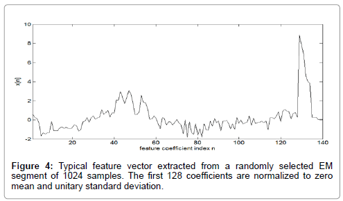
Figure 4: Typical feature vector extracted from a randomly selected EM segment of 1024 samples. The first 128 coefficients are normalized to zero mean and unitary standard deviation.
Figure 5 shows a randomly selected set of segments, assessed as successive fBm by the power-law wavelet method i.e. with r2>0.95 and 1 < b < 3. The R/S based Hurst exponents are shown against the segment index. The vertical axis starts at the minimum value, Hmin , of all the Hurst exponents of the dataset. Note, that this type of presentation ( Hmin -shift) waives the differences in the H-value range arising from the R/S analysis performed over different, one-month or longer, observation epochs in the EM time-series of the same or different recording stations, viz., time-series analyzed prior to different earthquakes or/and recorded by different stations. For comparison, we compute the Hurst exponents via the R/S method for the segments that do not exhibit fractal behavior (r2>0.95) or exhibit fractal behavior but not of the fBm kind (r2>0.95 and , shown in Figure 6. Because of their very large number, we pick a small sample of these, randomly spaced in time, and typically of size 1% of the total number and also compute their mean Hurst exponent, M. As it can be seen, the latter Hurst exponents of Figure 6 are lower when compared to the Hurst exponents of the successive fBm segments of Figure 5. According to section 2.4, a minimum threshold operator is applied on the Hurst exponents of successive fBm segments as a multiple of M. Figure 7 shows the Hurst exponents of the segments declared as successive fBm by the powerlaw wavelet method with a threshold set at 110% of M. Class I segments are the ones above the threshold while Class II segments are the ones below the threshold. The latter ones are grouped together with Class II segments of the cases with r2>0.95 or with r2>0.95 and ,as the ones shown in Figure 6. These segments, along with their class annotation, are used as training data for the SVM classifier.
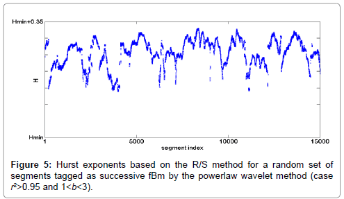
Figure 5: Hurst exponents based on the R/S method for a random set of segments tagged as successive fBm by the powerlaw wavelet method (case r2>0.95 and 1<b<3).
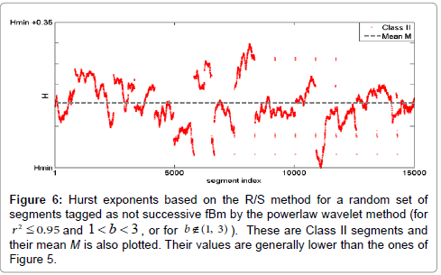
Figure 6: Hurst exponents based on the R/S method for a random set of segments tagged as not successive fBm by the powerlaw wavelet method (for r2 ≤ 0.95 and 1<b<3 , or for b €(1, 3) ). These are Class II segments and their mean M is also plotted. Their values are generally lower than the ones of Figure 5.
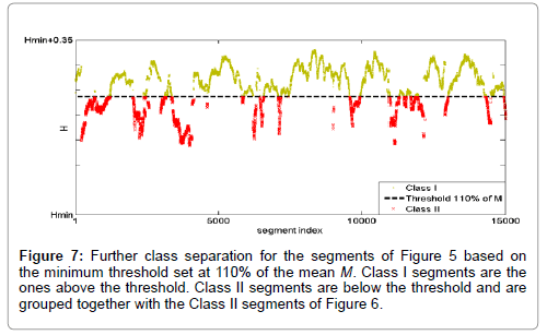
Figure 7: Further class separation for the segments of Figure 5 based on the minimum threshold set at 110% of the mean M. Class I segments are the ones above the threshold. Class II segments are below the threshold and are grouped together with the Class II segments of Figure 6.
The SVM classification results are presented and analyzed for each of the three earthquakes under investigation. The LIBSVM library [38] is employed in order to implement the SVM task. The EM measurement sequence of each earthquake is divided into training and testing data. The readings corresponding to the first five days of the 30-day monitoring process are used as training data for the computation of the SVM parameters. The remaining EM readings, corresponding to the next 25 days of monitoring, are allocated for testing and evaluating the SVM classifier. Table 1 describes the training and testing sets, in terms of number of segments, employed for each earthquake monitoring sequence. It is clear that the number of Class II segments is much higher than the number of Class I segments for all three cases. In order to have balanced training data, subsampling of the Class II segments in the time domain is employed such that the number of training segments of Class I and II is the same. For instance, the training set in the Crete 2009 recording is created by picking every 100th Class II segment in the time domain and all Class I segments, resulting in 9906 segments for both classes.
| Recording | Training Set (number of segments) | Testing Set (number of segments) | ||
|---|---|---|---|---|
| Class I | Class II | Class I | Class II | |
| Crete 2009 | 9906 | 9906 | 50794 | 2083606 |
| Crete 2013 | 1817 | 1817 | 97 | 2134303 |
| Limnos 2014 | 18007 | 18007 | 51559 | 2082841 |
Number of SVM training and testing segments for each class for all three 30-day earthquake monitoring periods. The training set corresponds to the first five days while the testing set to the remaining 25 days of each period
Table 1: Training and Testing Sets for SVM Classification.
The SVM parameters set is fine-tuned on the testing data of the three earthquakes by attempting to maximize the overall accuracy of the classifier on the testing set, given by
 (10)
(10)
After a coarse grid parameter search, a SVM kernel function that classifies the testing data with high overall accuracy is found to be an inhomogeneous polynomial of degree four, given as  with γ=1/140 and r=10. This kernel is used throughout the classification experiments. The individual class accuracy is given as
Accuracy rate for Class I (sensitivity), Class II (specificity) and overall accuracy rate corresponding to the entire 25 days period. The numbers in parentheses are the actual segment numbers that produce the percentage rates.
 (11)
(11)
The classification results are shown in Table 2. An overall accuracy rate of 90% or higher for all three monitoring sequences is attained. It can be observed that the SVM parameters set is fine-tuned towards higher accuracy in the classification of Class II segments rather than Class I segments, i.e., towards correctly identifying non-prominent segments rather than prominent segments. This also means that the particular SVM implementation is tailored towards minimizing the number of insignificant segments that are falsely declared as significant, i.e., the number of false alarms. This design choice also leads to high overall accuracy since the number of Class II segments is much higher than the number of Class I segments. Higher accuracy rates can be obtained for significant, Class I, segments at the expense of higher false alarm rates by selecting a different set of SVM parameters. Notice that since this is a binary classifier, the accuracy rate of Class I is identical to the sensitivity rate while the accuracy rate of Class II is identical to the specificity rate.
The class-specific, daily performance of the SVM for the 25 testing days is shown in Figure 8 for each of the three earthquakes. As explained before, the SVM accuracy for Class II segments is generally higher than for Class I segments. The earthquake sequences of Crete 2009 and Limnos 2014 contain Class I segments in all 25 monitoring days. The majority of the days observed in both earthquake sequences exhibit Class I accuracy of 80% or higher. The Crete 2009 sequence shows more than 90% accuracy in Class II segments for most of the 25 days tested while for the earthquake sequences of Crete 2013 and Limnos 2014, the same accuracy rate climbs above 95% in the majority of the testing days. The earthquake sequence of Crete 12/10/2013 presents a more peculiar case because the number of available Class I segments is very small, as seen in Table 1. According to Table 2, the actual number is only 97, compared to the 2.1x10⁶ segments of Class II. Nevertheless, the accuracy for both classes is very high even though the two classes are not represented in a balanced way in the testing set. Among the three cases, the earthquake of Crete 12/10/2009 posed the greatest classification challenge, as the Hurst exponents of Classes I and II are the closest in magnitude among the three earthquake sequences. The examples of Figures 3 and 4 actually depict this behavior for random samples derived from this particular earthquake sequence. Again, Class I Hurst exponents are higher than Class II Hurst exponents albeit this difference is not as high as in the other two earthquake sequences for which the SVM task is easier, as shown in Table 2. Further illustration for the lower SVM performance of Crete 2009 case as compared to the other two is provided by the Receiver Operating Characteristic (ROC) curves of Figure 9, computed on the testing data of the 25-day period. The larger the Area Under The Curve (AUC) is, the better the classification performance is in comparison. The AUC for the sequence of Crete 2009 is 0.9319, for the sequence of Crete 2013 is 0.9996 and for the sequence of Limnos 2014 is 0.9961. The best performance is attained for the case of Crete 2013 for which the AUC is almost one, i.e. the maximum possible value occurring in the case of perfect, error-free classification.
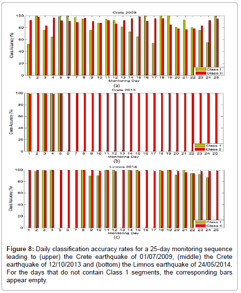
Figure 8: Daily classification accuracy rates for a 25-day monitoring sequence leading to (upper) the Crete earthquake of 01/07/2009, (middle) the Crete earthquake of 12/10/2013 and (bottom) the Limnos earthquake of 24/05/2014. For the days that do not contain Class 1 segments, the corresponding bars appear empty.
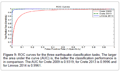
Figure 9: ROC curves for the three earthquake classification tasks. The larger the area under the curve (AUC) is, the better the classification performance is in comparison. The AUC for Crete 2009 is 0.9319, for Crete 2013 is 0.9996 and for Limnos 2014 is 0.9961.
| Recording | Accuracy Class I (sensitivity) % | Accuracy Class II (specificity) % | Overall Accuracy % |
|---|---|---|---|
| Crete 2009 | 83.9 (42603/50794) | 90.8 (1879777/2083606) | 90.1 (1922380/2134400) |
| Crete 2013 | 100.0 (97/97) | 99.7 (2128351/2134303) | 99.7 (2128448/2134400) |
| Limnos 2014 | 95.9 (49449/51559) | 98.6 (2054578/2082841) | 98.6 (2104027/2134400) |
Table 2: SVM Classification Results.
A novel algorithm on the detection of pre-seismic EM radiation anomalies was presented that fuses temporal long-memory analysis methods with SVM classifiers. In the fractal analysis stage, two previously deployed long-memory analysis methods were combined to jointly detect fractal anomalies in EM readings. A SVM classifier was trained on a fraction of these readings and then employed to verify and reproduce the fractal analysis detection results on the remaining data. Results for the long-memory analysis methods and the SVM classification stage were presented for three earthquake monitoring sequences recorded at three different locations and time instances in Greece. It was shown that the EM data separation into prominent fBm and non-prominent fBm or non-fBm parts performed by the two long-memory analysis methods is also reproducible by the SVM classifier by operating on features of the original EM data in a higher dimensional space. The SVM accuracy attained was 90% or higher for all three tested scenarios even though the three cases are very different in the occurrence pattern of Class I segments. The small computational complexity of the SVM decision process allows for real-time operation of the SVM classifier once its training is complete.
Conclusions
This paper constitutes an attempt of advanced analysis of EM signals collected prior to earthquakes in Greece. Three earthquakes, occurring at different locations and time instances, were selected as test cases to apply SVM classification techniques. The contribution of this work can be summarized as follows:
1.) The results of the analysis with power-law wavelet analysis and R/S method were presented. Significant pre-seismic segments were identified in all earthquakes by both long-memory analysis techniques and SVM methods. These segments were categorized as fBm profile.
2.) Results of the power-law wavelet analysis and R/S method were combined to identify the EM segments exhibiting high Hurst exponents and successive fBm profile. Several such segments were found in all three earthquake sequences under investigation.
3.) Results on SVM classification showed that the EM data separation into significant and insignificant parts performed by the two long-memory analysis methods is also reproducible by the SVM classifier by operating on reduced features of the original EM data. These features are of considerably smaller size as compared to the original data while the computational speed of the SVM allows for realtime implementation. The SVM accuracy attained was 90% or higher for all three tested scenarios.
Acknowledgement
The authors would like to thank Dr. Gregory Koulouras for the overall assistance for the maintenance of the EM network reported in this paper.
References
- Varotsos P, Alexopoulos K (1984) Physical properties of the variations of the electric field of the earth preceding earthquakes, I. Tectonophys 110: 73-98.
- Varotsos P, Alexopoulos K (1984) Physical properties of the variations of the electric field of the earth preceding earthquakes, II, determination of epicenter and magnitude. Tectonophys 110:99-125.
- Smirnova N, Hayakawa M, Gotoh K (2004) Precursory behavior of fractal characteristics of the ULF electromagnetic fields in seismic active zones before strong earthquakes. Phys Chem Earth 29: 445–451.
- Smirnova, N, Hayakawa M (2007) Fractal characteristics of the ground-observed ULF emissions in relation to geomagnetic and seismic activities. J AtmosSolar-Terrestrial Phys 69: 1833–1841.
- Hayakawa M, Hobara Y (2010) Current status of seismo-electromagnetics for short-term earthquake prediction. GeomaticsNat Hazard Risk 1:115-155.
- Eftaxias K (2010) Footprints of non-extensive Tsallis statistics, self-affinity and universality in the preparation of the L'Aquila earthquake hidden in a pre-seismic EM emission. Physica A 389: 133-140.
- Varotsos P, Sarlis N, Skordas E (2011) Scale-specific order parameter fluctuations of seismicity in natural time before main shocks.EPL(Europhysics Letters) 96 : 59002-p1/59002-p6.
- Kapiris P, Eftaxias K, Nomikos K, Polygiannakis J, Dologlou E, et al. (2003) Evolving towards a critical point: A possible electromagnetic way in which the critical regime is reached as the rupture approaches. Nonlinear Process Geophys10: 511–524.
- Eftaxias K, Contoyiannis Y, Balasis G, Karamanos K, Kopanas J, et al. (2008) Evidence of fractional-Brownian-motion-type asperity model for earthquake generation in candidate pre-seismic electromagnetic emissions. Nat Hazard Earth Syst Sci 8: 657-669.
- Eftaxias K, Athanasopoulou L, Balasis G, Kalimeri M, Nikolopoulos S, et al. (2009) Unfolding the procedure of characterizing recorded ultra-low frequency, kHz and MHz electromagnetic anomalies prior to the L’Aquila earthquake as pre-seismic ones – Part 1. Nat Hazard Earth Syst Sci 9: 1953-1971.
- Eftaxias K, Balasis G, Contoyiannis Y, Papadimitriou C, Kalimeri M, et al. (2010) Unfolding the procedure of characterizing recorded ultra low frequency, kHZ and MHz electromagnetic anomalies prior to the L’Aquila earthquake as pre-seismic ones - Part 2. Nat Hazard Earth Syst Sci 10: 275–294.
- Minadakis G, Potirakis S, Nomicos C, Eftaxias K (2012) Linking electromagnetic precursors with earthquake dynamics: An approach based on non-extensive fragment and self-affine asperity models. Physica A 391: 2232–2244.
- Potirakis S, Minadakis G, Eftaxias K (2012) Analysis of electromagnetic pre-seismic emissions using Fisher information and Tsallis entropy. Physica A 391: 300-306.
- Kapiris P, Polygiannakis J, Peratzakis A, Nomicos K, Eftaxias K (2002) VHF-electromagnetic evidence of the underlying pre-seismic critical stage. Earth Planet Space 54: 1237–1246.
- Stavrakas I, Clarke M, Koulouras G, Stavrakakis G, Nomicos C (2007) Study of directivity effect on electromagnetic emissions in the HF band as earthquake precursors: Preliminary results on field observations. Tectonophys 431: 263–271.
- Petraki E, Nikolopoulos D, Fotopoulos A, Panagiotaras D, Koulouras G, et al. (2013) Self-organised critical features in soil radon and MHz electromagnetic disturbances: Results from environmental monitoring in Greece. Appl Radiat Is 72: 39–53.
- Petraki E, Nikolopoulos D, Chaldeos Y, Coulouras G, Nomicos C, et al. (2014) Fractal evolution of MHz electromagnetic signals prior to earthquakes: results collected in Greece during 2009.Geomatics Nat Hazard Risk (in press).
- Yonaiguchi N, Ida Y, Hayakawa M, Masuda S (2007) Fractal analysis for VHF electromagnetic noises and the identification of preseismic signature of an earthquake. J AtmosSolar-Terrestrial Phys 69: 1825-1832.
- Kalimeri M, Papadimitriou C, Balasis G, Eftaxias K (2008) Dynamical complexity detection in pre-seismic emissions using non-additive Tsallis entropy. Physica A 387: 1161-1172.
- Eftaxias K, Panin V, Deryugin Y (2007) Evolution-EM signals before earthquakes in terms of meso-mechanics and complexity. Tectonophys 431: 273–300.
- Cicerone R, Ebel J, Britton J (2009) A systematic compilation of earthquake precursors. Tectonophys476: 371-396.
- Nikolopoulos D, Petraki E, Marousaki A, Potirakis S, Koulouras G, et al. (2012) Environmental monitoring of radon in soil during a very seismically active period occurred in South West Greece. J Environ Monitoring 14: 564-578.
- Nikolopoulos D, Petraki E, Vogiannis E, Chaldeos Y, Giannakopoulos P, et al. (2014) Traces of self-organisation and long-range memory in variations of environmental radon in soil: Comparative results from monitoring in Lesvos Island and Ileia (Greece). JRadioanalytical Nuclear Chem 299: 203-219.
- Madureira G, Ruano AE (2009) A neural network seismic detector. Acta Technica Jaurinensis 2: 159–170.
- Vallianatos F, Nomikos K (1998) SeismogenicRadioemissions as Earthquake Precursors in Greece. Phys Chem Earth 23: 953-957.
- Hurst H, Black R, Simaiki Y (1965) Long-term storage: an experimental study. Constable, London.
- Hurst H (1951) Long Term Storage Capacity of Reservoirs. Trans AmSoc Civil Engineers 116: 770-799.
- Lopez T, Martinez-Gonzalez C, Manjarrez J, Plascencia N, Balankin A (2009) Fractal Analysis of EEG Signals in the Brain of Epileptic Rats, with and without Biocompatible Implanted Neuroreservoirs. ApplMech Mater 15: 127-136.
- Dattatreya G (2005) Hurst Parameter Estimation from Noisy Observations of Data Traffic Traces, 4thWSEAS International Conference onElectronics, Control and Signal Processing, Miami, Florida, USA, 17-19 November, 193–198.
- Gilmore M, Yu C, Rhodes T, Peebles W (2002) Investigation of rescaled range analysis, the Hurst exponent, and long-time correlations in plasma turbulence. Phys Plasmas 9: 1312-1317.
- Rehman S, Siddiqi A (2009) Wavelet based Hurst exponent and fractal dimensional analysis of Saudi climatic dynamics. Chaos, Solitons and Fractals 39: 1081-1090.
- Kilcik A, Anderson C, Rozelot J, Ye H, Sugihara G, et al. (2009) Nonlinear prediction of solar cycle 24. Astrophys J 693: 1173–1177.
- Granero MS, Segovia JT, Perez JG (2008) Some comments on Hurst exponent and the long memory processes on capital markets. Physica A 387: 5543–5551.
- Eftaxias K, Kapiris P, Dologlou E, Kopanas J, Bogris N, et al. (2002) EM anomalies before the Kozani earthquake: a study of their behavior through laboratory experiments. Geophys Res Lett 29: 691-694.
- Eftaxias K, Kapiris P, Polygiannakis J, Bogris N, Kopanas J, et al. (2001) Signature of pending earthquake from electromagnetic anomalies. Geophys Res Lett 29: 3321–3324.
- Strang G, Nguyen T (1996) Wavelets and Filter Banks, Wellesley-Cambridge, USA.
- Chang CC, Lin CJ (2011) LIBSVM:a library for support vector machines. ACM Trans Intell Syst Technol 2: 1-27.
Citation: Cantzos D, Nikolopoulos D, Petraki E, Nomicos C, Yannakopoulos PH, et al. (2015) Identifying Long-Memory Trends in Pre-Seismic MHz Disturbances through Support Vector Machines. J Earth Sci Clim Change 6: 263. DOI: 10.4172/2157-7617.1000263
Copyright: ©2013 Cantzos D, et al. This is an open-access article distributed under the terms of the Creative Commons Attribution License, which permits unrestricted use, distribution, and reproduction in any medium, provided the original author and source are credited.
Select your language of interest to view the total content in your interested language
Share This Article
Recommended Journals
Open Access Journals
Article Tools
Article Usage
- Total views: 15677
- [From(publication date): 3-2015 - Jul 09, 2025]
- Breakdown by view type
- HTML page views: 10969
- PDF downloads: 4708