Utilization of Carbon in NPZ Model of Hooghly Estuarine System, India
Received: 31-Jul-2015 / Accepted Date: 17-Aug-2015 / Published Date: 22-Aug-2015 DOI: 10.4172/2157-7617.1000292
Abstract
Hooghly estuary along with the luxurious mangroves of the Sundarbans is one of the important estuaries of India. A quite rich mangrove patch in association with the creeks is visible at Sagar Island, the largest island in the row. Degradation and leaching of litter provides nutrient for the growth and development of phytoplankton which in turn strengthens the grazing food chain from zooplankton to fish. Phytoplankton growth is influenced by solar radiation, nutrient and temperature. The model incorporates light acclimation by algae, self-shading, photosynthetic production and nutrient uptake. Water quality changes with seasons. The model uses the functional relations among the three state variables as observed in response to the changeable environment throughout the year there. The model is calibrated and validated taking carbon as the currency of the model. Dissolved inorganic carbon as nutrient, water temperature, surface solar irradiance, and salinity of upstream and downstream of the estuary are collected from the field. Model results indicate that the growth of zooplankton and phytoplankton are enhanced by increasing nutrient input in the system. The predicted temporal distribution and trends of plankton biomass, inorganic carbon is in general agreement with field observations. Sensitivity analysis has been done. The model captures the dynamics of plankton population, which serve as major food source for fish species of the estuary. This model could be predictive in search for the role of mangrove in estuary and its control on nutrient and plankton dynamics of this region which will be helpful in management aspect.
Keywords: Mangrove, Sensitivity analysis, STELLA, Validation
11778Introduction
Rate of carbon fixation by phytoplankton is one of the most important biological processes and this is affected by a number of physical parameters. In spite of its huge impact on the whole living world, description on this aspect as a part of total carbon concentration has been scarce in literature till 1980s. But last two decades a number of works have been done on this topic in different ecological environments and depicting CO2 as limiting nutrient and also as a basic physiological autotrophic process. Since carbon dioxide (CO2) is the major greenhouse gas emitted by human activities, it is necessary to assess its sources and sinks, simulating the complex dynamics of CO2 flows involved in the carbon balance. Many researchers have studied the plankton dynamics along with nutrient fluctuation in different systems. They have proposed a number of nutrient (N)-phytoplankton (P)-zooplankton (Z), i.e., NPZ models. These models emphasized on different aspects of this dynamics. Simple NPZ model with simple equations [1] describing the nature of the system, gradually become complex model with incorporation of complexity at different level of the model. A ten compartment model by Fasham et al. [2], described the detailed equation for plankton dynamics. Dual currency is latest modification in NPZ models to understand the impacts of multinutrient on phytoplankton growth dynamics [3,4]. Edwards [5] studied the dynamics of two plankton population models to investigate the sensitivities of model complexity and introduced detritus to traditional NPZ models. Those models were aimed to study the dynamics (steady state and oscillations) of four state variables (NPZD) but lacked simulation using any particular set of data. Ray and Straskraba [6] constructed nutrient-phytoplankton-zooplankton-detritus-fish model of the Hooghly-Matla estuary and studied the dynamics of NPZD in the presence and absence of detritivorous fish in the system. They concluded that this group of fish had no impact on primary production but played a major role in the total fish production.
This work is done on the same Hooghly-Matla estuarine system and follows similar formulation of NPZ model as described in Ray and Straskraba [6] but excluding the fish compartment. Dynamic models are useful diagnosing the current state of the ecosystems, and for exploring how the system might respond to future changes in environmental factors.
This work describes the structure and dynamics of a nutrient, phytoplankton, and zooplankton model for the estuarine system near Sagar Island. The model tracks the flow of nutrient (inorganic carbon) from the bottom of the food web (phytoplankton) to zooplankton which includes copepods, cyclopods, rotifers, some fish larvae etc. Higher order predators in the system are not directly incorporated as state variables in the model. Field data of environmental factors as forcing functions are used to simulate this model. This work is the extension of the previous work [7] where a simulation dynamic model is constructed describing the role of litrerfall of the adjacent mangrove forest as a source of nutrient (carbon) supply in this estuarine system. The objectives of the present work are to know – (i) the dynamic behaviour of plankton throughout the year in relation to the nutrient supply, (ii) the dynamics of nutrient and plankton in relation with environmental factors.
Materials and Methods
Description of study area
Sundarbans, vast lash green mangroves with distinctive faunal diversity, is located along the coastal line of Bay of Bengal, where the Ganges meets the sea (Figure 1). A wide variety of fishes harbour in the whole estuarine area and so the livelihood of the local people is mainly dependent on this ecosystem. The Sundarbans, a unique bioclimatic zone, is expanded over the borders of two countries- India and Bangladesh. A number of rivers, creeks and canals perforate the areas like a network [6,8]. Hooghly estuary, a meso-macrotidal estuary shows a wide mixing zone extending from Diamond Harbor to the mouth of the river [9]. Sagar Island, the largest deltaic island in this estuarine complex, lying between 21°56′–21°88′ N and 88°08′–88°16′ E is located in the western sector of the estuary. The island is about 144.9 km2 in area, and is surrounded by the river Hooghly on the north and northwest and the river Mooriganga on the east [10]. South western wind controls the monsoon here. During premonsoon when the river run off is low, temperature remains high and salinity is also very high. With the arrival of the monsoon nutrient and suspended matters are increasing.
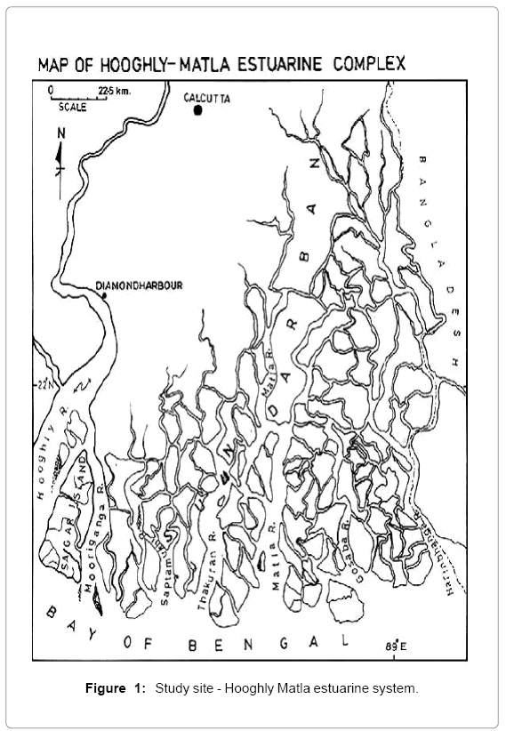
Figure 1: Study site - Hooghly Matla estuarine system.
This region is under the wet tropical climatic zone, with pronounced seasonal climatic changes. The seasons can be divided into pre-monsoon (March–June) with average high temperature ranging from 27–46°C and minimum rainfall; monsoon (July–October), when about 80% of annual rainfall occurs, and post-monsoon (November–February), with cold weather (average 23°C) and negligible rainfall. The monsoon season is generally dominated by southwest winds. The average humidity is about 80% and more or less uniform throughout the year. Avicennia marina (grey mangrove) is the dominant species among the halophytes of Sagar Island. Avicenna alba, Porteresia coarctata, Excoecaria agallocha, Ceriops decandra, Acanthus ilicifolius and Derris trifoliate are also present [11].
Experiments
Samples are collected from the creeks of Sagar Island. Some experimental and survey works are done over two years in the field to collect data for water temperature, water pH, dissolved inorganic carbon (DIC), water temperature, salinity, etc.
Plankton are collected from surface water using a plankton net during high tide, and preserved with Lugol’s iodine solution (phytoplankton) or buffered formaldehyde (zooplankton). For quantitative analysis of phytoplankton, wet and dry weights are measured and phytoplankton carbon content is calculated following the literature [12]. For zooplankton carbon, the Sedgewick Rafter counting method is employed to obtain the number of organisms and the corresponding carbon content is estimated following standard method [13].
Description of model
To observe the dynamics of NPZ throughout the year, STELLA 6.0 computer software (High Performance System Inc.) is used to construct a 3-state variable model (Figure 2). The model is integrated by using fourth-order Runge–Kutta method with a time step of 1 day. Carbon (mgC/l) is considered as currency in the model. Dissolved inorganic carbon (DIC) in estuary is contributed by various sources and converted to other forms of carbon [7]. In the creeks of Sagar Island, input of DIC to the system (Inp) is through various sources like diffusion of CO2 at air-water interface, conversion from Soil Inorganic Carbon and Soil Organic Carbon to DIC loss of nutrient, respiration of plankton (Rp and Rz). DIC is converted to other forms of carbon (Cp) depending on pH of water. Phytoplankton uptake DIC during photosynthesis (U). DIC is removed from the system during tidal flash (L1). Dynamics of DIC is stated in equation 1.
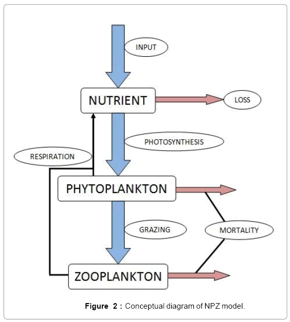
Figure 2: Conceptual diagram of NPZ model.
 (1)
(1)
 (1.1)
(1.1)
 (1.2)
(1.2)
 (1.3)
(1.3)
 (1.4)
(1.4)
 (1.5)
(1.5)
 (1.6)
(1.6)
Uptake of DIC by phytoplankton during photosynthesis is described in equation 1.5. Nutrient uptake by algae is generally described by a Michaelis-Menten (Type II) equation with the half- saturation constant serving affinity of phytoplankton for a particular nutrient [14]. Dynamics of phytoplankton in the estuary is balanced by uptake of DIC during photosynthesis(U), grazing by zooplankton (G), respiration (Rp), natural mortality (Mp) and settling (S) and loss from the system (L2) (Eq 2).
 (2)
(2)
 (2.1)
(2.1)
 (2.2)
(2.2)
 (2.3)
(2.3)
 (2.4)
(2.4)
 (2.5)
(2.5)
 (2.6)
(2.6)
Michaelis–Menten kinetics is followed for grazing of zooplankton on phytoplankton (G). Phytoplankton (P), zooplankton (Z), and half saturation constant for phytoplankton grazing by zooplankton (Kz) are included in the grazing equation. G is also dependent on dilution (D) and grazing rate of zooplankton (grt) (Eq. 2.1). Because estuary is a transition zone of river and sea, there is always fluctuation of salinity throughout the year, which is because of dilution or mixing of water. D is calculated, equations (2.2) and (2.3), following [15], where f is the dilution factor, Sr is salinity of upstream, and Se is salinity of downstream.
 (3)
(3)
 (3.1)
(3.1)
 (3.2)
(3.2)
 (3.3)
(3.3)
 (3.4)
(3.4)
Besides grazing, the abundance of zooplankton is also dependent on respiration (Rz), loss because of fish predation (Pr), and mortality (Mz), excretion (Ex) and loss from the system during tidal flush (L3) (equation 3). All the parameter values and the initial values of the state variables are listed in Tables 1-3.
| State Variables | Value | Unit | Reference | |
|---|---|---|---|---|
| DIC | Dissolved Inorganic Carbon pool | 225 | mgC/l | Field survey |
| P | Phytoplankton | 0.39 | mgC/l | Field survey |
| Z | Zooplankton | 0.48 | mgC/l | Field survey |
Table 1: Description, initial values, units and references of the state variables of
the model.
| Graph Time Functions | Value | Unit | Reference | |
|---|---|---|---|---|
| InpDIC | Conversion rate of DIC to DBC | Graph | dimensionless | Field survey |
| Se | Conversion rate of DIC to DCO2 | Graph | dimensionless | [17] |
| Sr | Conversion rate of DBC to DCO2 | Graph | dimensionless | [17] |
Table 2: Description, values, units and references of the graph time functions of the model.
| Forcing Functions | Value | Unit | Reference | |
|---|---|---|---|---|
| Ppsyn | Photosynthesis rate | 1.0002 | day-1 | Calibrated |
| kDIC | Half saturation constant for nutrient uptake by phytoplankton | 0.05 | day-1 | [12] |
| rCP | Rate of conversion of DIC to other forms of carbon | 0.43 | day-1 | Calibrated |
| mrP | Mortality rate of phytoplankton | 0.234 | day-1 | [12] |
| rphy | Respiratory rate of phytoplankton | 0.024 | day-1 | [12] |
| lrt1 | Loss rate of nutrient | 0.49 | day-1 | Ray, 2008 |
| srt | Settling rate of phytoplankton | 0.15 | day-1 | [12] |
| lrt2 | Loss rate of phytoplankton | 0.156 | day-1 | Roy et al., 2012 |
| rex | Excretion rate of zooplankton | 0.01 | day-1 | [12] |
| rZoo | Respiratory rate of zooplankton | 0.025 | day-1 | [12] |
| grt | Growth rate of zooplankton | 0.6 | day-1 | [12] |
| kZ | Half saturation constant for phytoplankton grazing by zooplankton | 0.02 | day-1 | [12] |
| prZ | Rate of predation by fish | 0.22 | day-1 | Ray et al., 2002 |
| mrZ | Mortality rate of zooplankton | 0.15 | day-1 | [12] |
| lrt3 | Loss rate of zooplankton | 0.18 | day-1 | Roy et al., 2012 |
Table 3: Description, values, units and references of the forcing functions of the model.
Sensitivity analysis
All the parameters are considered for sensitivity analysis which is the fundamental step before calibration. Sensitivity analysis attempts to provide a measure of the sensitivity of either parameters, or forcing functions, or submodels to the state variables of greatest interest in the model. Sensitivity analysis is performed using the following formula: S=(dx/x)/(dp/p) (Jorgensen, 1994), where S=sensitivity, x=state variable (here, DIC, P and Z), p=parameter, dx and dp are change of values of state variables, parameters and forcing functions respectively. Those parameters, which are almost impossible to calculate from field are calibrated using a range of values (minimum to maximum) collected from literature first and further the appropriate value for that parameter for this estuary are determined according to the best fit of the value during the model run by using standard calibration procedure [16].
Model calibration and validation
Calibration is done by adjusting selected parameters in the model to obtain a best fit between the model calculations and the field data collected during first year of study period. Validation of the model is performed using data collected during second year of study period. The monthly average values of the state variables of first year and second year are used for calibration and validation of the model respectively. The model is simulated for the period of 365 days.
Results
Model result indicates that the state variable DIC is sensitive to ppsyn, rtCP and lrt1 (Table 4). If rCP is increased and decreased 10% then DIC is increased or decreased by 4.5% and 4.8%, respectively. If lrt1 is changed (increase and decrease) by 10%, DIC values change by about 5%. If Ppsyn is increased and decreased by 10% DIC increases 1.6% and 3.6%, respectively. Few forcing functions (grt, kZ, rex and prZ) which are not sensitive at 1% level show little sensitivity when forcing functions are changed at 10% level. But the values are low, always below 0.5%. The variation of DIC throughout the year ranges between 140–320 mg/l. Field observations show DIC concentrations are higher in premonsoon (210–320 mg/l) and lower in monsoon (140–183 mg/l). Chi-square value for observed and simulated results of DIC shows that the discrepancy is not significant. Phytoplankton dynamics is directly proportional and highly sensitive to Psyn, rCP, kDIC, lrt1, grt. The range of the state variable P throughout the year is very narrow. The value is lowest in monsoon due to the facts that during monsoon water column remains turbid and light penetration is lowered and also availability of DIC is lowered, so, growth of phytoplankton is diminished. Cyanophyta, Green algae, Euglenophyta, Dinophyta, Bacillariophyta, and Pinnate are different groups comprising of phytoplankton population. It is reported that not all these groups are encountered at a time rather representative genus of these groups appears at different seasons throughout the year [9,17]. In post monsoon (November to February), the phytoplankton growth is enhanced by favorable environmental conditions like less turbid water, sufficient surface solar irradiance, and adequate nutrient availability in the estuary [18]. Zooplankton population mainly consists of cyclopod, rotifers and copepods. Seasonal variation does not show very distinct in their abundance throughout the period of study. In premonsoon (March to June), zooplankton biomass reaches its highest value in April (0.515 mgC/l) whereas their population decreases during monsoon (July to October) and reaches its lowest value in October (0.319 mgC/l). Chi-square value for observed and simulated results of Z is 0.20 (p<0.05). Zooplankton dynamics is highly sensitive to rCP, lrt3, kDIC, mrZ, Ppsyn and prZ. In premonsoon, the zooplankton in the estuary is very high which in turn also reduces the phytoplankton population (Figure 3).
| Forcing Functions | DIC | Phytoplankton | Zooplankton |
|---|---|---|---|
| rCP | 0.338 | 0.138 | 0.175 |
| lrt1 | 0.043 | 0.209 | 0.148 |
| Psyn | -0.796 | 1.030 | 0.946 |
| rphy | 0.000 | 0.000 | 0.000 |
| kDIC | 0.000 | 0.002 | 0.006 |
| rzoo | 0.000 | 0.000 | 0.005 |
| lrt2 | 0.000 | 0.000 | 0.000 |
| srt | 0.000 | 0.000 | 0.000 |
| mrP | 0.000 | 0.000 | 0.000 |
| grt | 0.000 | 0.750 | 0.294 |
| kZ | 0.000 | 0.000 | 0.000 |
| rex | 0.000 | 0.000 | 0.002 |
| prZ | 0.000 | 0.156 | 0.394 |
| mrz | 0.000 | 0.215 | 0.068 |
| lrt3 | 0.000 | 0.116 | 0.078 |
Table 4: Result of sensitivity analysis.
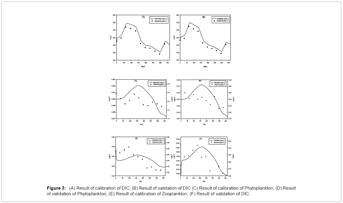
Figure 3: (A) Result of calibration of DIC; (B) Result of validation of DIC (C) Result of calibration of Phytoplankton; (D) Result of validation of Phytoplankton; (E) Result of calibration of Zooplankton; (F) Result of validation of DIC.
Equilibrium solutions and stability of the model
(i) The first equilibrium of the system is Nutrient only equilibrium point  (
( ), where InpDIC > rcp and when the rate of dissolved inorganic carbon (DIC) in estuary (InpDIC) is more than the DIC conversion to other forms of carbon (Cp) ( InpDIC > rcp ), then this equilibrium point is feasible and in this situation if the per-capita phytoplankton mortality rate due to different causes (
 ) is higher than its percapita growth
  i.e.,
i.e., , then system settles down to Nutrient only steady state ( ) (Appendix A). It is quite obvious that, if phytoplankton’s mortality due to different causes is higher than its growth rate, then with increasing time, phytoplankton naturally goes to extinction and zooplankton automatically suffers and is also eliminated. The input rate of dissolved inorganic carbon in estuary is more than its conversion to the other forms of carbon hence; DIC is increased unless the condition is changed.
(ii) The second equilibrium point of the system is zooplankton free equilibrium point (
( ),
),
where  and
and  . This equilibrium point is feasible if
  and either
  or
or  , where
  and
and
 Under this circumstances if the loss rate of zooplankton due to all causes ( prz + rex + rzoo + mrz + lrt3 ) is more than its growth rate
  i.e.
i.e.  and loss rate of phytoplankton by all means except zooplankton consumption
  is more than its growth rate
  i.e.
i.e.  , the system shows zooplankton free equilibrium (Appendix A). By remaining the condition fixed, the stability of zooplankton free equilibrium point
  (
( ) describes that the loss rate of zooplankton is higher than its growth rate; the zooplankton is eliminated from the system. In the absence of zooplankton, DIC and phytoplankton shows equilibrium state, initially in that condition phytoplankton increases but up to its carrying capacity and perhaps equilibrium point stays around carrying capacity. But when zooplankton is present in the system, the whole system also shows equilibrium state and here it might in the equilibrium point lies between the carrying capacity of phytoplankton.
(iii) The third and most important equilibrium is the coexistence equilibrium point  ,
,
where  ,
,  and
and  is the unique positive root of
This equilibrium point is locally asymptotically stable if  and
and  (Appendix A). Figures of equilibrium point are depicted in Figure 4.
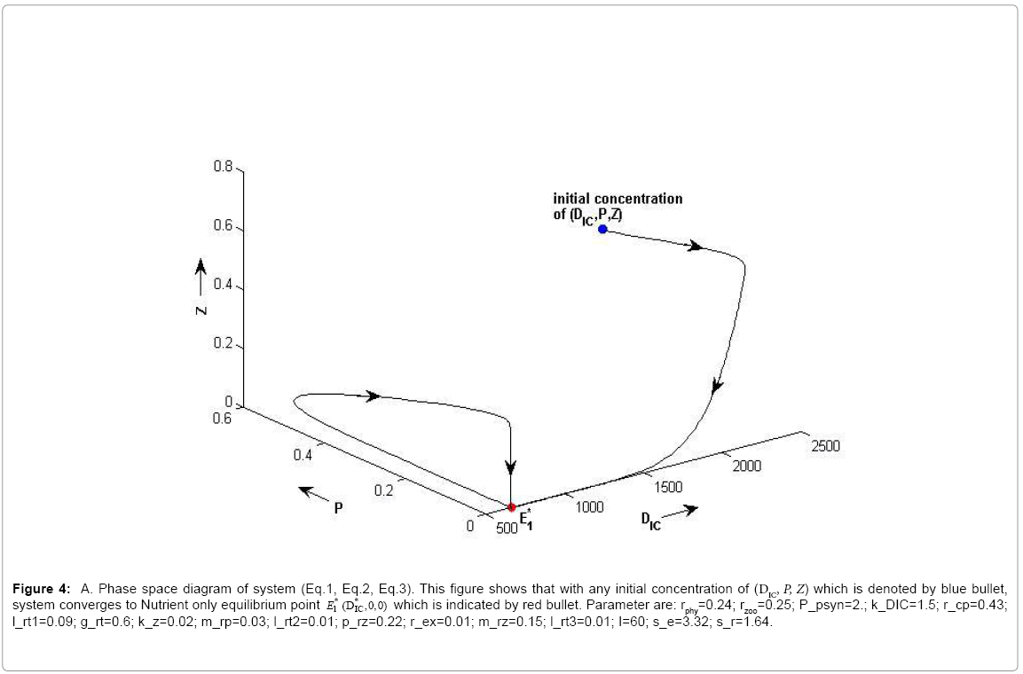
Figure 4a: A. Phase space diagram of system (Eq.1, Eq.2, Eq.3). This figure shows that with any initial concentration of (DIC, P, Z) which is denoted by blue bullet,system converges to Nutrient only equilibrium point E*1(DIC,0,0) which is indicated by red bullet. Parameter are: rphy=0.24; rzoo=0.25; P_psyn=2.; k_DIC=1.5; r_cp=0.43; l_rt1=0.09; g_rt=0.6; k_z=0.02; m_rp=0.03; l_rt2=0.01; p_rz=0.22; r_ex=0.01; m_rz=0.15; l_rt3=0.01; I=60; s_e=3.32; s_r=1.64.
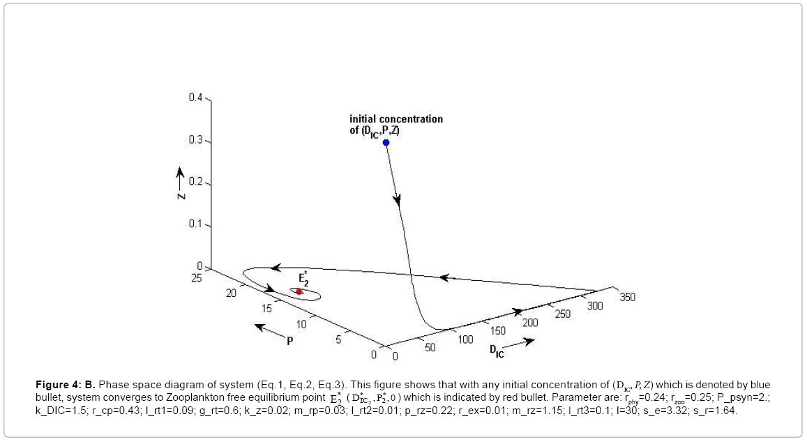
Figure 4b: B. Phase space diagram of system (Eq.1, Eq.2, Eq.3). This figure shows that with any initial concentration of (DIC, P, Z) which is denoted by blue bullet, system converges to Zooplankton free equilibrium point () which is indicated by red bullet. Parameter are: rphy=0.24; rzoo=0.25; P_psyn=2.;k_DIC=1.5; r_cp=0.43; l_rt1=0.09; g_rt=0.6; k_z=0.02; m_rp=0.03; l_rt2=0.01; p_rz=0.22; r_ex=0.01; m_rz=1.15; l_rt3=0.1; I=30; s_e=3.32; s_r=1.64.
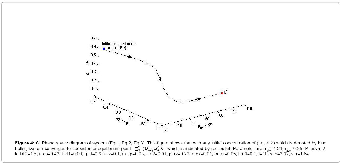
Figure 4c: C. Phase space diagram of system (Eq.1, Eq.2, Eq.3). This figure shows that with any initial concentration of (DIC, P, Z) which is denoted by blue bullet, system converges to coexistence equilibrium point * E*2 DIC ,P2 ,0 ) which is indicated by red bullet. Parameter are: rphy=1.24; rzoo=0.25; P_psyn=2; k_DIC=1.5; r_cp=0.43; l_rt1=0.09; g_rt=0.6; k_z=0.1; m_rp=0.03; l_rt2=0.01; p_rz=0.22; r_ex=0.01; m_rz=0.05; l_rt3=0.1; I=10; s_e=3.32; s_r=1.64.
Discussion
Anthropogenic activities and ongoing climate change are posing stress to the coastal environment affecting the ecology of phytoplankton which is responsible for about 15% of global oceanic production. Fluctuations in river flow, stratification of the water column, grazing pressure by zooplankton, nutrient dynamics, and light availability control the phytoplankton bloom in shallow estuaries [9]. This estuary is highly disturbed due to nutrient load from river discharge which result from economic growth in areas of reclaimed from mangrove forest [19].
Anthropogenic nutrient input from the Hooghly–Matla estuary to the creeks of Sagar Island varies between 0.257 mg/l and 0.390 mg/l annually [19]. Apart from anthropogenic input of nutrient, the biomass of phytoplankton and zooplankton are directly related to litter production of the adjacent mangrove forest [17]. Salinity plays as an important factor determining zooplankton dynamics in Hooghly– Matla estuary [20]. Gradation of salinity along the estuarine area is dependent on the dilution factor which is a function of mixing fresh water from river and the saline water from sea. The salinity drops down where it meets river and its value increases along the stretch toward the sea. Salinity-dependent dilution is calculated following the method of [15]. In the monsoon months, salinity decreases considerably (2.04– 5.16 ppt) because of heavy rains and higher fresh water input. This pattern is also shown by Biswas et al. [9]. As a result, only those species which are able to withstand lower salinity condition can establish themselves in the creeks [20]. During monsoon the river experiences a huge amount of fresh water input carrying significant amount of nutrient load. But at that time due to turbidity light penetration is lower causing poorer productivity and growth of plankton. The highest primary production is observed during premonsoon when nutrient availability is good and also light penetration is the most in the water column. It differs from the Godavari estuary where primary production in the system is mainly controlled by light availability in the water column than nutrients [21]. As the freshwater input is decreased and the transparency is increased due to reduction in suspended solids, phytoplankton bloom is developed. Similar result is also obtained in the study of phytoplankton over two decades in this estuary by Biswas et al. [9]. During post monsoon, sufficient nutrient encourages plankton growth. Besides, during monsoon, the area remains inundated with water which creates anoxic conditions beneath the water column and releases CO2. Photosynthetic rate of marine algae as function of inorganic carbon concentration using Michelis Menten equation has been discussed by Caperon and Smith [22]. Similar equations are used in models [23,24].
Phytoplankton biomass is lower in monsoon than pre and post monsoon. Therefore, rainfall is a factor determining plankton dynamics. Similar trend is also evident from previous studies [9]. Higher primary productivity is observed during the summer season, because of high population density of phytoplankton. As the salinity and other hydrological parameters are in stable condition during summer the phytoplankton production remain high. Perumal et al. [18] proposed that this higher density could also be due to neritic element domination, higher salinity and surface water temperature, clear water conditions besides availability of nutrients. The recorded low primary productivity could be related to the wash of the phytoplankton to the neritic region by the monsoonal flood besides reduction of salinity, which could have affected the phytoplankton population [25-27]. During monsoon, high amount of allochthonous input is very high as river runoff in the estuary. This input causes high turbidity in the estuarine water which retards phytoplankton growth. The observed low zooplankton productivity during monsoon might be due to the nonavailability of food, low temperature and low salinity. The disturbances of the food web and minimum production of plankton during the monsoon season have been observed in many Indian estuaries [28,29]. Owing to the inflow of freshwater during the monsoon, the salinity of the water column decreases. The low salinity would drastically affect the plankton abundance [30]. In the present investigation, increase or decrease of salinity in the water column exerts either a direct or an indirect effect in the appearance or disappearance of some forms and replacement by others. This phenomenon is introduced in the model as salinity based grazing equation of zooplankton.
Conclusion
To avoid the mathematical complexity of the model, only essential parameters are dealt with in this model. After successful calibration and validation, the model seems to be realistic. This region is very important for the production of commercially important fisheries. Productivity is dependent on nutrient availability in the creeks of the Hooghly–Matla estuarine system. This model is able to predict the present status of plankton dynamics, which serve as major food resource for herbivorous and carnivorous fish species.
Acknowledgments
One of the authors (JM) is thankful to University Grants Commission (UGC), Govt. of India, New Delhi for providing RFSMS fellowship as financial support to carry out this work and Institute of Environmental Studies and Wetland Management (IESWM), Saltlake, Kolkata for giving the opportunity to carryout experiments on their laboratories. JM is also thankful to Mr. Jalad Gayen for his assistance in the collection of samples during field surveys for this work.
Conflict of Interest
The authors have no conflict of interest whatsoever.
References
- Steele JH, Henderson EW (1981) A simple plankton model. Am Nat 676-691.
- FashamMJR, DucklowHW, McKelvicSM (1990) A nitrogen-based model of plankton dynamics in the oceanic mixed layer. J Mar Res 48:591-639.
- Flynn KJ (2003) Modelling multi-nutrient interactions in phytoplankton;balancing simplicity and realism. ProgOceanogr 56: 249-279.
- Mitra A (2006) A multi-nutrient model for the description of stoichiometric modulation of predation (SMP) in micro- and mesozooplankton. J Plankton Res 28: 597-611.
- Edwards AM (2001) Adding detritus to a nutrient-phytoplankton-zooplankton model: a dynamical-systems approach. J Plankton Res 23: 389-413.
- Ray S, Straskraba M (2001) The impact of detritivorous fishes on a mangrove estuarine syste m. Ecol Model 140: 207-218.
- Mukherjee J, Ray S, Ghosh PB (2013)A system dynamic modeling of carbon cycle from mangrove litter to the adjacent Hooghly estuary, India. Ecol Model 252: 185-195.
- Biswas H, Mukhopadhyay SK, De TK, Sen S, Jana TK (2004) Biogenic Controls on the Air-Water Carbon Dioxide Exchange in the Sundarban Mangrove Environment, Northeast Coast of Bay of Bengal, India. LimnolOceanogr 49: 95-101.
- Biswas H, Dey M, Ganguly D, De TK, Ghosh S, Jana TK (2010) Comparative Analysis of Phytoplankton Composition and Abundance over a Two-Decade Period at the Land-Ocean Boundary of a Tropical Mangrove Ecosystem. Estuaries Coasts 33: 384-394.
- Mandal S, Ray S,Ghosh PB (2009) Modelling of the contribution of dissolved inorganic nitrogen (DIN) from litterfall of adjacent mangrove forest to Hooghly-Matla estuary, India. Ecol Model 220: 2988-3000.
- Saha S, Choudhury A (1995) Vegetation analysis of restored and natural mangrove forest in Sagar Island, Sundarbans, east coast of India. Indian J Mar Sci24:133-136
- JorgensenLA, JorgensenSE, NielsenSN (2000) ECOTOX, Ecological Modelling and Ecotoxicology. Elsevier, Netherlands.
- FriedlerE, JuanicoM, ShelefG (2003) Simulation model of wastewater stabilization reservoirs. Ecol Eng 20: 121-145.
- Eppley RW, Coatsworth JL, Solorzano L (1969) Studies of nitrate reductase in marine phytoplankton. LimnolOceanogr 14: 194-205.
- Ketchum BH (1951) The exchange of fresh and salt water in tidal estuaries. J Mar Res 10: 18-38.
- Jorgensen SE (1994) Fundamentals of Ecological Modelling(2ndedn.) Elsevier, Netherlands.
- MandalS, RayS, GhoshPB (2012) Modeling Nutrient (Dissolved Inorganic Nitrogen) and Plankton Dynamics at Sagar Island of Hooghly-Matla Estuarine System, West Bengal, India. Nat Resour Model 25: 629-652.
- PerumalN, Vengadesh M, Rajkumar P, Perumal K, Rajasekar T (2009) Seasonal variations of plankton diversity in the Kaduviyar estuary, Nagapattinam, southeast coast of India. J EnvBiol30: 1035-1046.
- Mukhopadhyay SK, Biswas H, De TK, Jana TK (2006) Fluxes of nutrients from the tropical river Hooghly at the land-ocean boundary of Sunderbans, NE Coast of Bay of Bengal. India. J Mar Syst 62: 9-21.
- Bhunia AB Ecology of Tidal Creeks and Mudflats of Sagar Island (Sunderbans) West Bengal (1979) Doctoral dissertation, Calcutta University.
- Sarma, VVSS, Prasad VR, Kumar BSK, Rajeev K, Devi BMM, Reddy NPC, Sarma VV, Kumar MD (2010) Intra-annual variability in nutrients in the Godavari estuary, India. Continental Shelf Research 30: 2005-2014.
- Caperon J, Smith DF(1978) Photosynthetic rates of marine algae as a function of inorganic carbon concentration. LimnolOceanogr23: 704-708.
- Meersche Van den K, Middelburg J, Soetaert K, van Rijswijk P, Boschker H, Heip C (2004) Carbon-nitrogen coupling and algal-bacterial interactions during an experimental bloom:Modeling a 13C tracer experiment. LimnolOceanogr49: 862-878.
- Chen C, Ji R, Schwab DJ, Beletsky D, Fahnenstiel GL, Jiang M, Lavrentyev PJ (2002) A model study of the coupled biological and physical dynamics in Lake Michigan. Ecol Model 152: 145-168.
- Rajasegar M, Srinivasan M Rajaram R (2000) Phytoplankton diversity associated with the shrimp farm development in Vellar estuary, south India. Seaweed Res Utiln 22: 125-131.
- Gowda G, Gupta TRC, Rajesh KM, Gowda H, Lingadhal C Ramesh AM (2001) Seasonal distribution of phytoplankton in Nethravathi estuary, Mangalore. J Mar Biol Ass India 43: 31-40.
- ThillaiRajsekar K, Perumal P, Santhanam P (2005) Phytoplankton diversity in the Coleroon estuary, southeast coast of India. J. Mar. Biol Ass India 47: 127-132.
- Kannan R, Kannan L (1996) Physico-chemical characteristics of seaweed beds of the Palk bay, Southeast coast of India. Indian J Mar Sci 25: 358-362.
- Satpathy KK (1996) Seasonal distribution of nutrients in the coastal waters of Kalpakkam, East Coast of India. Indian J Mar Sci25: 221-224.
- Godhantaraman N (1994) Species composition and abundance of tintinnids and copepods in the Pichavaram mangroves (South I ndia). Cienc Mar 20: 371-391.
Citation: Joyita M, Debaldeb J, Moitreyee B, Bhusan PG, Santanu R (2015) Utilization of Carbon in NPZ Model of Hooghly Estuarine System, India 6: 292. DOI: 10.4172/2157-7617.1000292
Copyright: © 2015 Joyita M, et al. This is an open-access article distributed under the terms of the Creative Commons Attribution License, which permits unrestricted use, distribution, and reproduction in any medium, provided the original author and source are credited.
Select your language of interest to view the total content in your interested language
Share This Article
Recommended Journals
Open Access Journals
Article Tools
Article Usage
- Total views: 17015
- [From(publication date): 8-2015 - Jul 19, 2025]
- Breakdown by view type
- HTML page views: 12335
- PDF downloads: 4680