Research Article Open Access
Ecosystem Approach to Fisheries and Marine Ecosystem Modelling: Review of Current Approaches
Stecken M and Failler P*Economics and Finance Group, Portsmouth Business School, University of Portsmouth, Richmond Building, Portland Street, Portsmouth, PO1 3DE, UK
- *Corresponding Author:
- Failler P
Economics and Finance Group, Portsmouth Business School
University of Portsmouth, Richmond Building, Portland Street
Portsmouth, PO1 3DE, UK
Tel: +44 (0)2392 848 505
Fax: +44 (0) 2392 844 614
E-mail: pierre.failler@port.ac.uk
Received Date: July 26, 2016; Accepted Date: August 10, 2016; Published Date: August 30, 2016
Citation: Stecken M, Failler P (2016) Ecosystem Approach to Fisheries and Marine Ecosystem Modelling: Review of Current Approaches. J Fisheries Livest Prod 4: 199 doi: 10.4172/2332-2608.1000199
Copyright: © 2016 Stecken M, et al. This is an open-access article distributed under the terms of the Creative Commons Attribution License, which permits unrestricted use, distribution, and reproduction in any medium, provided the original author and source are credited.
Visit for more related articles at Journal of Fisheries & Livestock Production
Abstract
This paper presents a review of existing approaches on ecosystem modelling and assesses them in the light of their capacity to integrate main elements of the ecosystem and their pertinence for fishery management. It completes existing EAF reviews by adding substantial analysis of the way to incorporate ecosystem complexities in models. The two most used approaches use nearly the same structure of boxes with flows of biomass for EwE or flows of elements for BM2. The main difference which gives a more efficient modelling is the method of estimates coming from the steady state model ECOPATH. This method is one of the strength of the EwE approach giving it a good predictive power. However, it is in the same time one of its main weakness in assuming an equilibrium situation that is far to be always the case. BM2 and biogeochemical models in general will have a better predictive power for low trophic levels. The problem in raising trophic levels is the higher number of parameters which raises in the same time the uncertainty of such models. The last model, ECGEM, is a recent model with an original approach. It presents, however, several important weaknesses as its ecological pertinence remains to be proved. Despite this, the model requires less parameters and supply methods needed by standard models and thus allows to process more complex situations.
Keywords
Ecosystem; Biodiversity; Biomass; Biogeochemical; Planktivorous
Introduction
Ecosystem Approach to Fisheries (EAF) attained official international recognition in 2001 during the Reykjavik Conference on Responsible Fisheries in the Marine Ecosystem organised by the government of Iceland and the FAO. This was reinforced during the Johannesburg Plan of Implementation (JPoI) in September 2002 after the EAF has been indicated indispensable for marine biodiversity conservation. More recently, in September 2006 during the Bergen conference, EAF has become a necessary step towards sustainable management of Fisheries.
In Parallel to the EAF, ecosystem-level models were being developed such as Ecopath (EwE), biogeochemical models initiated in the 80’s or more recently Ecological Computable General Equilibrium Model (ECGEM) in the late 90’s. Currently, the two firsts have become main approaches used to model marine ecosystem due to their availability while being in perpetual development. The EwE initiated by Polovina, was further developed by Christensen and Pauly [1] while biogeochemical models were originally constructed to model interactions between organisms of low trophic levels. Biogeochemical models such as ERSEM [2,3] have progressively raised the number of trophic levels such that it has been eventually considered as ecosystem models. The ECGEM proposed by Tschirhart [4] is a recent parallel approach between marine ecosystem and economic market. Their goals are different, but with similar baselines such as to characterize species, their relations to each other and the interaction of species with their natural environment towards a proper interpretation of the ecosystem.
This paper presents a review of existing approaches on ecosystem modelling and assesses them in the light of their capacity to integrate main elements of the ecosystem and their pertinence for fishery management. It completes existing EAF reviews by adding substantial analysis of the way to incorporate ecosystem complexities in models. The first part of this paper presents the main characteristics of the models. The second part provides an analysis of their capacity to imitate real ecosystem functioning. A third part is a discussion on the pertinence of the EAF for fishery management. A conclusion gives the main findings.
Models Presentation
The three approaches of ecosystem modelling are presented and analysed through three representative models. The most popular model and software that relies on the allocation of biomass in discrete groups is the mass balanced Ecopath model [1,5,6] and its timedynamic extension Ecosim [7,8]. The present paper limited its focuses on the time dynamic representation of the ecosystem while the spatial component Ecospace, [9] of the software will not be addressed here. The second type of model described in the paper is the ECGE model [4,10,11] which describes an ecosystem as an economic market. The third type of model studied will be the biogeochemical models where the Bay model 2 (BM2) [12] has been chosen as representative model among the numerous existing biogeochemical models due to its capacity of describing the whole ecosystem, not only the lower trophic level. It is simpler than IGBEM [13], which is derived from ERSEM II, and has been the subject of several studies, which makes it a good tool to compare with the two initial models mentioned.
EwE approach
Ecopath: Ecopath estimates trophic flows between the different components of the ecosystem. Each component is represented as a box that contents species or an aggregation of species having a common physical habitat, similar diet, and similar life history characteristics [5].
The Ecopath model is based on two master equations which describe this balance:
Biomass balance for the group i:

Bi is the biomass of group i
Pi for each group i
Yi the total fishery catch rate of i,
M2i is the instantaneous predation rate for group i
Ei the net migration rate (emigration − immigration),
BAi is the biomass accumulation rate for i,
M0i is the ‘other mortality’ rate for i.
Energy balance for the group i:
Consumption(i)=production(i)+respiration(i)+unassimilated food(i). (EwE-2)
From these two equations, the linear equation at the base of Ecopath is given as:
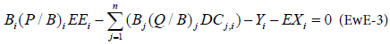
For an ecosystem with n species groups, the resolution of a system of n linear equations allows estimating for each equation, with one unknown variable among the Biomass, the P/B ratio (production/ biomass), the C/B ratio (consumption/biomass) and the Ecotrophic Efficiency, which is the is the proportion of the production that is utilized in the system described as:

It can be noted that for a system assumed closed (no emigration), the ratio (P/B)i is equal to the total mortality rate Zi, which is often more accessible to the Ecopath user [6,14]
Ecosim
Ecosim is the dynamic version of Ecopath. It has been described by Walters [7] to give a dynamic representation of the ecosystem. Ecosim expresses biomass dynamics through a series of coupled differential equations. The equations are derived from the Ecopath master Eq. (1) and takes the form:
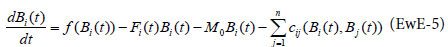
with the functions:
f(Bi(t)): Biomass production in absence of predation
cj(Bi(t), Bj(t)) : Biomass of prey i consumed by predator j at time t.
Fi(t)Bi(t)) : Fishing losses
M0Bi(t): Natural mortality
It will be seen later how these functions are expressed
ECGEM
The ecological computable general equilibrium model has been described by Tschirhart [4] and Finnoff and Tschirhart [10]. The objectives of this model are to describe an ecosystem in the same way as an economic market with energy price as signal. A parallel can be drawn between the economic market and an ecosystem considering individuals as firm and species as industries. The price that regulates the trade is the energy price paid by individuals to receive energy. It is assumed that non human individuals behave rationally and maximize their net energy intake, hence population adjustments are derived. To proceed, the ecosystem is divided in m specie groups (with p < m plants species), and each biomass transfer is assumed to take place in a biomass market. The main equation of this model is the expression for the net energy for an individual of specie i:
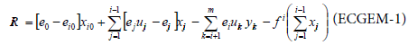
ei: energy per unit of biomass coming from j (j=0→ coming from sun)
eij: energy spent to capture and locate a unit of biomass of specie j by i.
xij,yij: flow of biomass
uij: parameter to represent the fact that predators are often unsuccessful to catch their prey (uij<1)
The term on the right hand side of the equation above is the energy from the Sun. The second term is the energy inflow coming from consumption, the third one represents the energy outflow, and the two last ones represent respiration losses. All these terms are analysed more accurately in the second part of this paper.
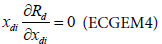
The variables of this model are demands xij and prices eij. A short run equilibrium is obtained by solving the following equations:
-The equilibrium conditions: supply=demand for every market
-The derivatives of equation ECGEM1 with respect to the demands equal to zero for every species group considered in the ecosystem.
An example treated in Tschirhart [4], considered a system of 14 equations and 14 variables. From the value of Ri, it is described how the evolution of the population number is modelled.
Bio-geochemical model
BM2 is a biogeochemical ecosystem model which tracks the nitrogen and silicon pools of 25 living, 2 dead, 4 nutrients and 6 physical components. It was built to replace the detailed process equation used for each invertebrate group in the IGBEM with the general form of the process equations implemented for the biological components in the Port Phillip Bay integrated model [15]. This model used to describe the Port Phillip Bay [12]. This bay is divided into 59 geometric boxes vertically resolved (water column, epibenthic, sediment). For each modelled group, a rate of change in equation is defined which is a function of the different ecosystem process modelled. The different ecosystem processes are summarised in the following Table 1.
| Different Pools | Process describing this rate |
|---|---|
| Autotrophs | growth/natural mortality/predation |
| Invertebrate Consumers | growth/natural mortality/predation/fishing losses |
| Fish Consumers | growth/natural mortality/predation/fishing losses |
| Inanimate Pools | uptake/inflow/nitrification/denitrification |
| Detritus | waste/natural mortality/consumption of detritivores |
Table 1: Ecosystem process.
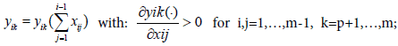
Each type includes several different groups, for example the fish consumers regroup the planktivorous, piscivorous, demersal and demersal herbivorous fishes. For each of these groups, the rate of changed equations and the processed equations will have the same structure but different rates; this is precisely described in Fulton [13].
The solving of this model is made with a daily time-step wherever it is possible, however, such a time scale may make the variables with fast dynamics become unstable. Therefore, some groups use an adaptive time-step. Once this has occurred the transport model steps are performed and a run can be performed.
Modelling of the ecosystem complexity: Methods and analyse of what?
In a marine ecosystem, the primary production is the process which depends in the biggest way of physical parameters. Thus the primary production done by photoautotroph will be dependent of parameters such as irradiance, nutrient concentration, temperature. The modelling of this process is then directly linked to the capacity to incorporate such physical parameters in the models. However, the modelling of this process cannot be done efficiently if knowledge on this part of the ecosystem is not sufficient.
The way to incorporate such parameters influence in the model is presented and analysed according to their capabilities to integrate ecosystem complexity. Thus we will consider how the physical parameters seen above are modelled. The first difference between the three models is the time step. The time step is directly linked to model capabilities to catch ecosystem complexity. BM2 uses a daily time step whereas ECGEM uses a yearly one. EwE time step depends of the EwE user choice. The large time step used by ECGEM represents a strong weakness for the ECGEM which won’t be able to catch ecosystem seasonality.
Primary production in the net energy equation for a primary producer i is expressed as:
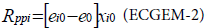
xi0: biomass fixed by i
ei0: solar energy fixed per unit biomass of xi0
e0: energy price spent to fix xi0
The resolution of the equation systems explained in section I.2 gives the value of xi0 and e0.
This equation is a difference between the energy assimilated by the plants under the form of biomass: ei0xi0, and the energy spent by the plant to fix the former energy; e0xi0. This equation represents the energy inflow for each plant species i, and consequently the energy inflow for the whole ecosystem.
The drawback of this process in the model is due to different limitations as abiotic factors or by competition phenomenon is translated in the model by an increase of the price paid to fix energy. This idea to make the price ei0 a function of other species population or the abiotic factors is mentioned by Tschirhart [4]. However, no example of function has been enounced, and besides the ecological pertinence of such a formulation is still to prove. More work is needed to validate ecologically this way to the primary production.
According to Finnoff and Tschirhart [10], no chemoautotroph groups are modelled. This omission is an important weakness for an ecosystem model. However, we can assume that this modelling could be appended by adding one or several chemoautotroph groups and defining the energy price adapted.
EwE and BM2 model the primary production explicitly for each group of producers as a function of the population group. In BM2, the limitation of nutrient, light and space for the expressions see, [13] are explicitly modelled.

With μPX the maximum growth rate, δirr the irradiance limitation factor, δN the nutrient limitation factor due to nitrogen, δspace the space limitation factor.
EwE uses to model primary production a basic function with density dependence.

ri: maximum P/B that (i) can exhibit when Bi is low
ri/hi is the maximum net primary production rate for pool (i) when biomass (i) is not limiting to production (Bi high).
These parameters are estimated from the values of ECOPATH parameters. The estimate of hi from ECOPATH assumes that the system is close to the equilibrium. The explicit limitation of nutrient loading has been added [6] to EwE through the Michaelis-Menten uptake relationship:
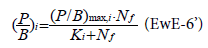
Nf being the quantity of free nutrient on the ecosystem. It comes from estimates of the total inflow rate and total losses of nutrient and from a constant proportion between free nutrient and fixed nutrient.
A new idea is being developed by Christensen and Walters [6] to incorporate parameters as salinity or concentration of elements. It consists to add in the model a group which will represents one of this parameters. The variation of this new group is modelled by a forced function. The relation between characteristic of primary producers and this parameter has to be defined by a function or an equation determined empirically for the modelled ecosystem. This way to proceed allows EwE to model these parameters. This application of the idea is still being under development, and once it will be done BM2 and EwE will integrate physical factors in a similar way.
Concerning the modelling of the primary production, ECGEM is clearly less accurate than the two other models. BM2 and EwE have the capabilities to incorporate parameters influence as luminosity and nutrients concentration. The primary production process can be considered as well modelled by these two models.
Consumption
The analysis of modelling consumption in an ecosystem will be based upon the study of the functional responses which are used in the models. The functional response is a core structural feature of a trophodynamic model [16]. As said by Yodzis [17], its mathematical form represents the researcher’s view of the biological details of that particular predation process and profoundly affects model behaviour. By studying the different functional responses used in these three models we will be able to analyse how this process is modelled and what ecosystem complexity it allows to incorporate in the model.
Functional response representation
The functional response of EwE and BM2 can be clearly expressed thanks to the formulation of these two models.
For Ecosim, the consumption function is the following:
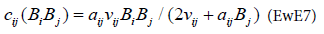
This equation is based on the foraging arena concept explained by Walters [7]. This concept assumes the existence of two pools of biomass for the same prey, one available to the predator, the other being unavailable with a rate of change between these two pools of vij (scheme).
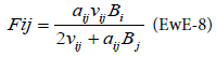
The parameters aij and νij are estimates from the Ecopath model. The functional response derived from this consumption equation is:
In BM2, the consumption equation is used in the process equation representing the growth of consumers:

The term Pi,CX represents the amount of biomass transferring from the prey i to the consumer CX. In a standard run of BM2, the functional response used is a Holling type 2 response:
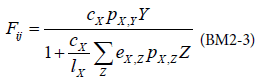
with X representing the predator, Y, the preys.
cX: maximum clearance rate
pX,Y: availability of prey Y to predator X
eX,Z: assimilation efficiency of predator X on prey Z
lX: maximum growth rate of predator X
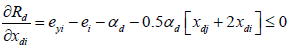
For the ECGEM, the functional response is not explicitly modelled because the CGE approach determines consumption and densities of both predator and prey. Therefore, for Tschirhart [11] tracking functional response is first a matter of deciding what the appropriate response to track. Tschirhart [11] determines what possible response by determining the sign of the following derived:
 and
and  with xd:biomass flow from the prey to the predator and Ny the number of prey. Details of this analysis are described by Tschirhart [11] and his conclusion is that for a number of fixed predator, which is the assumption used during the short run equilibrium, and the consumption of fixed prey (Nyxy=cst), the ECGEM models consumption as a type II Holling response.
Functional response analysis: To analyse these different functional responses used to model the consumption process, it will be seen firstly what are the phenomenon implicitly modelled by these responses. Then, we will consider the efficiency of these responses to reproduce real ecosystem (Figure 1).

Figure 1: Simulation of flow between available (Vi) and unavailable (BiVi) prey biomass in Ecosim. ai is the predator search rate for prey i, is the exchange rate between the vulnerable and un-vulnerable state (Walters, 1997).
The two main phenomena leading to the consumption process in a marine ecosystem are the availability of the prey to predator and the choice of the predator between different preys. The availability can be illustrated by the example cited by Walters [7]; planktivorous fish often spend much of their time in behavioural (schooling) or spatial (shallow water, holes) refuges that limit their encounter rates with (or the time they are exposed to) piscivores. This phenomenon is modelled in EwE and BM2, through a constant. However, these constants do not have the same representations and applications in the two models. The BM2 availability constant is presented as the numerator of the functional response (BM2-3) and with a value between 0 and 1, it reduces the consumption rate.
For EwE, the availability term was vij described above. It is assumed that the exchange process between V and B operates on short time scales relative to changes in Bi and Bj. Consequently, Vij should stay near the equilibrium as implied by setting dV/dt=0, which allows to predict the consumption equation seen above (EwE-7). The way to estimate vij from Ecopath is described in Walters [7]. This method of estimation allows one to have realistic estimates, however, the equilibrium hypothesis of Ecopath make these estimates realistic only for an ecosystem close to the equilibrium situation.
The ECGEM method to represent the availability of prey is not explicitly described in the different publications [4,10,11]. However, its method to describe the paid price to catch a prey allows it to incorporate in this price an availability factor. But this factor will be confronted to the same problem of estimation as the one of BM2.
The prey selection is a preponderant phenomenon in ecosystem life. However, this phenomenon is difficult to model due to the diversity of potential preys and the complex selective behaviour of the predator. In EwE, this process although preponderant, is not modelled. The diet composition matrix, which represents the proportion of prey consumed by predators, is used to estimate the consumption rate Qij in Ecopath from which the aij and vij are derived. These parameters stay constant in each run.
For BM2, the prey selection influence is incorporated in the denominator of the functional response (BM2-3) by expressing the following sum: 
With eX,Z: assimilation efficiency of predator X, pX,Z: availability of prey Z to predator X, Z: biomass of prey. This sum allows to make the prey consumption Y decreases or increases according to the consumption of other preys.
In Tshirhart [11] analyses the modelling of this phenomenon. To proceed, he considers a fictive system with two preys of the same predator. Applying the net energy equation (ECGEM3) and the Kuhn- Tuncker optimality conditions (ECGEM4), the ECGEM will predict the consumption of one prey only if the marginal energy gained per biomass unit consumed equals the sum of marginal energy loses to locating, attacking handling i and to marginal respiration.


The functional form of respiration is expressed under a quadratic form (ECGEM3) which is, according to Tshirhart, reasonably general to be used, however it can be estimated given enough data. The ei and ej will change with changing densities leading to switching in the proportion of prey consumption by the maximisation of Rd (ECGEM3).
In the nature, the variation of other prey consumption will vary the predator selection, that’s what is modelled in BM2 and in ECGEM. But it’s far to be the only cause in predator selection. Another important cause which can be cited is the exposure risk to predators of the individual preying on its prey. This idea is not include in the BM2 model. In Finnoff [10] models this factor by making for a species i the consumed outflow a function of the consumption inflow. Thus in the net energy equation (ECGEM-1), we have:

In the general net energy equation, the fact to link the consumption outflow to the consumption inflow is a way to link exposure to the risk to be consumed.
The way to model the consumption process with a more or less accurate level has been made for the three different approaches. We have to say that the ECGEM, being a recent model, needs more studies in order to determine the ecological pertinence of such an approach. However, the way it is used at present to describe ecosystem presents interesting elements, especially for its choice of predator modelling
To conclude this part on the consumption process modelling, the main weaknesses and strengths of these models can be cited. For EwE, its strength is in its availability factor estimated from Ecopath. ECGEM models availability as well by determining the price to pay and the unsuccessfulness factor: uij. However, these parameters are much harder to estimate than those of EwE to which the estimation are realistic for an ecosystem in equilibrium situation.
BM2 doesn’t model this availability phenomenon, this is its most important weakness. The other important phenomenon regulating the consumption process is the selection of a prey by a predator. The fact to not take this into account represents an important weakness for EwE. According to Yodzis [17], this is consequently not truly multispecific.
BM2 and ECGEM consider both the prey selection by predator. BM2 considers it in the expression of its functional response (see above) and ECGEM does it with its energy maximisation hypothesis. To be validate ecologically, ECGEM needs a lot of work, however, this approach could be a different way which would need much less parameter estimation [18-20].
Detritus
The detritus cycle is the last basic trophic process occurring in marine ecosystem. To describe the detritus modelling, the inflows and outflows will be considered separately. These inflows are constituted by the waste of the consumption process and by the mortality of ecosystem individuals and outflows by the detritivore consumption.
The incorporation of the cited inflow parameters will be presented in a matrix (Table 2), following by the description of this modelling. Secondly, the modelling of recycling of detritus will be analysed in the same way as for the analysis of the consumption process.
| Detritus inflows | Waste of consumption | Mortality |
|---|---|---|
| ECGEM | - | - |
| EwE | + | + |
| BM2 | + | + |
Table 2: Parameters taken into account in the modelling of detritus inflows.
The evaluation of parameters is made according to four possibilities:
+: explicitly modelled
- : not modelled
The first thing that can be noticed is the fact that ECGEM does not consider any detritus compartments. Consequently, even if the respiration terms represent a loss of biomass which is translated in loss of energy, that one is considered as lost in the atmosphere and non reusable in the ecosystem. This omission is an important weakness for an ecosystem model.
EwE and BM2 represents both inflows due to both mortality and waste consumption. The difference between EwE and BM2 comes from the way to integrate these inflows.
Inflows due to waste of consumption
The waste of consumption is modelled in EwE and BM2. However, in EwE models this process in a much simpler way as does BM2.
EwE uses a default parameter (20%) coming from Winberg (1956) to estimate the waste of consumption flows. This parameter can be change if the user wishes so. BM2 models this waste in the same way by using the parameter ΓXX.(1-εXX). There is one ΓXX.(1-εXX) for each type of consumption; on living prey, on labile detritus, on refractory detritus (see the following equation, BM2-4)
The structure of BM2 is more complex.
For example, the equation representing the waste products sent to the labile detritus:

(BM2-4)
The three first term in the brackets represents the waste products sent to detritus when feeding respectively on live prey, on labile detritus, on refractory detritus, with ΓXX.(1-εXX).PXX representing the proportion of the growth inefficiency of XX sent to detritus. The last term in the brackets represent the proportion of mortality losses assigned to detritus. fXX, DL is the proportion of the total detritus produced that is of the type DL. The same equation is used for the production of DR except that fXX, DL is replaced by (1-fXX, DL). So for this point, there is no structural difference between these two models.
Inflows due to mortality
The second inflow which can be considered is the inflow due to species mortality. In EwE this term is represented by the term M0Bi (EwE5) representing the mortality not accounted for by the predation in the system. This flow determined with Ecopath estimates is entirely directed to the detritus box.
In BM2, the term of mortality directed to the detritus boxes is taken into account in the equation above (BM2-4) and is written as follow:

(BM2-5)
This equation regroups linear and mortality term representing respectively the basal mortality and the mortality due to predators not modelled; the mortality term due to oxygen dependence applying only for benthic feeder groups; the ‘special’ mortality which represents different exceptional mortalities (stress/fouling by epiphytes/ starvation); the last term is the mortality due to top predators. The proportion of the total mortality assigned to the detritus is represented by the term φXX (BM2-4).
BM2 models differently the mortality of the primary producers by the following equation of lysis mortality:
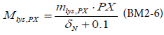
with mlys,PX the rate of lysis and δN the limitation factor due to nitrogen.
Knowing every inflow terms, the rate of change equation for detritus is given:
For the labile detritus of the water column:
 (BM2-7)
with the following successive terms: waste of invertebrate consumers, waste of fish consumers, waste of pelagic bacteria, lysis of primary producers, lysis of microphytobenthos, mortality of macroalgae, recycling due to pelagic attached bacteria, recycling due to benthic feeders. In the same model, the rate of change equation is described in Fulton [13] for the different detritus boxes.
The first remark which can be done is the different complexity levels of these two models. The quantity of parameters to estimate will be much more important for BM2 than for EwE. Moreover, the estimation method of the EwE package gives a better pertinence in the parameters value than those of BM2. The second essential process of the detritus dynamic which allows the recycling of biomass in the ecosystem is the consumption of detritus. This process is made by detritivores groups as bacteria, several benthic feeders or some fish species. The modelling of this process is done in EwE by the inclusion in the model of this detritivore groups and then the consumption is modelled as any other consumption flow with the equation EwE-7.
In BM2 this recycling is described in the equation above with the terms PDLw,PAB and PDLw,BF which represents the biomass of DLw which is consumed by pelagic attached bacteria and benthic feeders respectively. No function is cited for these consumption expressions.
Conclusion
This paper has described three different approaches which model marine ecosystems. The two most used approaches use nearly the same structure of boxes with flows of biomass for EwE or flows of elements for BM2. The main difference which gives a more efficient modelling is the method of estimates coming from the steady state model ECOPATH. This method is one of the strength of the EwE approach giving it a good predictive power. However, it is in the same time one of its main weakness in assuming an equilibrium situation that is far to be always the case. BM2 and biogeochemical models in general will have a better predictive power for low trophic levels. The problem in raising trophic levels is the higher number of parameters which raises in the same time the uncertainty of such models. The last model, ECGEM, is a recent model with an original approach. It presents, however, several important weaknesses as its ecological pertinence remains to be proved. Despite this, the model requires less parameters and supply methods needed by standard models and thus allows to process more complex situations.
It is important to notice that good predictive power is not a foregone conclusion with ecosystem models (NPRB website): the systems are extremely complex, and the data available for fitting, tuning and testing models are very sparse relative to the spatial, temporal and taxonomic details of the models and of the system. Because of this difficulty, there is a trade off between ecosystem complexity integration and the number of parameters which makes increase the uncertainty.
Several fields of work are necessary to improve modelling capacity; the ecosystem knowledge, the data harvesting, the ecosystem complexity modelling are the three main fields. This paper has presented the different ways used to incorporate this complexity. By trying to make an objective evaluation of these ways, this paper gives options for future modelling and indicates basically the main points which needs improvement.
Acknowledgements
This paper has been carried out with financial support from the Commission of the European Communities, specific RTD programme ‘‘International Research in Co- operation’’ (INCO-DEV), ‘‘Ecosystems, Societies, Consilience, Precautionary principle: development of an assessment method of the societal cost for best fishing practices and efficient public policies’’ (ECOST). It does not necessarily reflect its views and in no way anticipates the Commission’s future policy in this area.
References
- Christensen V, Pauly D (1992) ECOPATH II - A software for balancing steadystate ecosystem models and calculating network characteristics. Ecological Modelling 61: 169-185.
- Baretta JW, Ebenhoh W (1995) The European regional seas ecosystem model, a complex marine ecosystem model Netherlands. Journal of Sea Research 33: 233-246.
- Bekker BJG, Baretta JW, Ebenhöh W (1997) Microbial dynamics in the marine ecosystem model ERSEM II with decoupled carbon assimilation and nutrient uptake. Journal of Sea Research European Regional Seas Ecosystem Model II 38: 195-211.
- Tschirhart J (2000) General Equilibrium of an Ecosystem. Journal of Theoretical Biology 203: 13-32.
- Polovina JJ (1984) Model of a coral reef ecosystems. I. The ECOPATH model and its application to French Frigate Shoals. Coral Reefs 3: 1-11.
- Christensen V, Walters CJ (2004) Ecopath with Ecosim: methods, capabilities and limitations. Ecological Modelling Placing Fisheries in their Ecosystem Context 172: 109-139.
- Walters C, Christensen V, Pauly, D (1997) Structuring dynamic models of exploited ecosystems from trophic mass-balance assessments. Rev. Fish Biol. Fish 7: 139-172.
- Walters C, Pauly D, Christensen V, Kitchell JF (2000) Representing density ependent consequences of life history strategies in aquatic ecosystems. EcoSim II Ecosystems 3: 70-83.
- Pauly D, Christensen V, Walters C (2000) Ecopath, Ecosim, and Ecospace as tools for evaluating ecosystem impact of fisheries. J Mar Sci 57: 697-706.
- Finnoff D, Tschirhart J (2003) Harvesting in an eight-species ecosystem. Journal of Environmental Economics and Management 45: 589-611.
- Tschirhart J (2004) A new adaptive system approach to predator-prey modeling. Ecological Modelling 176: 255-276.
- Smith ADM, Johnson CR (2004) Biogeochemical marine ecosystem models I: IGBEM-a model of marine bay ecosystems. Ecological Modelling 174: 267-307.
- Fulton EA, Parslow JS, Smith ADM, Johnson CR (2004) Biogeochemical marine ecosystem models II: the effect of physiological detail on model performance. Ecological Modelling 173: 371-406.
- Pauly D, Moreau J (1995) Comparison of age-structured and length-converted catch curves of brown trout Salmo trutta in two French rivers. Fisheries Research 22: 197-204.
- Murray A, Parslow J (1997) Port Phillip Bay Integrated Model: Final Report. Technical Report No. 44. Port Phillip Bay Environmental Study. CSIRO, Canberra, Australia.
- Yodzis P (1994) Predator-prey theory and management of multispecies fisheries. Ecol Appl 4: 51-58. 17.
- Yodzis P (2005) Multispecies modelling of some components of the marine community of northern and central Patagonia, Argentina. Published on the NRC Research Press.
- Fulton EA, Smith ADM, Johnson CR (2003) Mortality and predation in ecosystem models: is it important how these are expressed? Ecological Modelling 169: 157-178.
- Walters C, Pauly D, Christensen V (1999) Ecospace: prediction of mesoscale spatial patterns in trophic relationships of exploited ecosystems, with emphasis on the impacts of marine protected areas. Ecosystems 2: 539-554.
- Winberg GG (1956) Rate of metabolism and food requirements of fishes. Transl Fish Res Board Can 194: 1-253.
Relevant Topics
- Acoustic Survey
- Animal Husbandry
- Aquaculture Developement
- Bioacoustics
- Biological Diversity
- Dropline
- Fisheries
- Fisheries Management
- Fishing Vessel
- Gillnet
- Jigging
- Livestock Nutrition
- Livestock Production
- Marine
- Marine Fish
- Maritime Policy
- Pelagic Fish
- Poultry
- Sustainable fishery
- Sustainable Fishing
- Trawling
Recommended Journals
Article Tools
Article Usage
- Total views: 3902
- [From(publication date):
December-2016 - Aug 29, 2025] - Breakdown by view type
- HTML page views : 2932
- PDF downloads : 970