Evaluation of Upland Rice Genotypes and Mega Environment Investigation Based on GGE-Biplot Analysis
Received: 05-Apr-2017 / Accepted Date: 19-Jul-2017 / Published Date: 25-Jul-2017 DOI: 10.4172/2375-4338.1000183
Abstract
Though a recent introduction, rice is becoming the most important food and cash crop in Ethiopia. However, its productivity is being constrained mainly by lack of improved varieties. Identification of high yielding and stable genotype(s) and desirable environment(s) has been the most important objectives of multi-environment trials. The objectives of the present study were to explore the effect of genotype and genotype × environment interaction on grain yield of upland rice genotypes and to examine the possible existence of different mega environments. Grain yield performances of 13 upland rice genotypes were evaluated under rainfed conditions at three locations (Woreta, Pawe, Metema) in North Western Ethiopia from 2011 to 2013. The study was laid out in a randomized complete block design with three replications. The first two principal components (IPC1 and IPC2) were used to create a twodimensional GGE biplot that accounted for 76.80% and 20.05%, respectively. A combined analysis of variance showed that both main effects (environment and genotype) and GE interactions were highly significant. The polygon tool of the biplot suggested the existence of two upland rice mega-environments with wining genotypes G3, G9, G8 and G12. Visualizing the mean and stability parameters of the genotypes in the biplot indicated that genotypes NERICA-13 (G3), FOFIFA-3730 (G11) and NERICA-12 (G2) are adapted to rainfed upland rice growing areas of North Western Ethiopia. According to the ideal-genotype biplot, genotypes G3 followed by G2 and G11 were better genotypes demonstrating their high mean yield and stability performance.Based on discrimination and representation, Woreta was identified as the ideal location for generally adaptable upland rice genotypes and Metema for selecting specifically adaptable upland rice genotypes. Finally, it was concluded that genotypes; G2, G3 and G11 showed high grain yield and stability performance across environments and were promoted to variety verification. Of which, G2 has been officially released for large scale production with the common name “NERICA-12’’.
Keywords: G × E interaction; GGE biplot analysis; Mega environment; Multi-environment trials; NERICA rice
35434Introduction
Among the target commodities that have received due attention in promotion of agricultural production, rice (Oryza sativa L.) is expected to contribute in ensuring food security in Ethiopia [1]. Though introduced recently, the importance of rice as food and cash crop is being well recognized as the demand for rice, the trend of area coverage, and the number of rice producers and processors is increasing in different parts of the country. However, lack of improved varieties is one of the most pressing constraints in rice production and productivity in the country where rice breeding is found at infant stage. As a result, there is a wide gap between demand and supply which needs to bridge the gap through developing improved varieties.
Towards this end, the national rice improvement research project has been actively involved in developing varieties through multi environment trials. However, the multi-environment trial (MET) usually results in genotype-by-environment interactions (GEI). GEI refers to differential ranking of genotypes across environments and may complicate the selection process and recommendation of a genotype for a target environment [2]. This interaction is the result of changes in genotype’s relative performance across environments due to differential responses of the genotypes to various edaphic, climatic and biotic factors [3]. In a GEI, measured traits are less predictable and cannot be interpreted using main effects and need more analysis. GEI is also one of the most important reasons for the failure and/ or decreased efficiency of breeding efforts to serve resource-poor farmers.
Information on the structure and nature of GEI is particularly useful to breeders for it can help to determine if they need to develop cultivars for all environments of interest or if they should develop specific cultivars for specific target environments. Yan [4] indicated that analysis of genotype–by-environment data from multienvironment trials has been an important component of plant breeding to select favorable genotypes based on both mean yield and stability and to determine whether a test environment is homogeneous or should be divided into various mega-environments.
The detection of GEI has led to the development of different statistical models to describe GE interaction. These models have been classified as univariate versus multivariate approaches [5]. Unlike that of univariate ones, multivariate statistical approaches explore multidirectional aspects of GEI and attempt to extract more information from GE interaction components [3,6]. Genotype plus genotype by environment interaction biplot (GGE biplot) analysis is one of the multivariate statistical models and a new technique for graphical display of GE interaction pattern of MET data with many advantages [7,8]. It is an effective tool for mega-environment analysis, genotype and environmental evaluation. It has been proposed that GGE biplot analysis was a useful method for the analysis of GE interactions and had been exploited in the variety evaluation of wheat [7], maize [9] and rice [10].
This is the first attempt in Ethiopia to classify upland rice production into mega environments (ME), assessing the discriminating ability and representativeness of test environments and identifying high yielding and stable genotypes based on multi environment grain yield data. Sub division of crop growing region into several mega-environments helps in allocation of resources in a breeding program, target genotype distribution to appropriate production area, and information exchanges between breeding programs [11]. Therefore, this study was conducted to interpret the magnitude and causes of genotype (G), environment (E) and GE interaction on yield performances of upland rice genotypes, to examine the possible existence of different mega environments and the wining genotype for each mega environment, to evaluate the yield performance and stability the genotypes and to assess the discriminating ability and representativeness of the testing locations.
Materials and Methods
Planting materials and trial management
Thirteen upland rice genotypes (Table 1) were evaluated at three locations (Woreta, Pawe and Metema) of six environments (E) including E-1(Woreta-2011), E-2 (Pawe-2011), E-3 (Woreta-2012), E-4 (Pawe-2012), E-5 (Woreta-2013) and E-6 (Metema-2013) from 2011 to 2013 under rainfed conditions. The locations where the study was conducted differ in their agro ecological characters (Table 2). Randomized complete block design (RCBD) with three replications was used.
| Genotype | Source | Locationsvs.Grain yield | Mean | |||
|---|---|---|---|---|---|---|
| Name | Code | Woreta | Pawe | Metema | ||
| NERICA-11 | 1 | Africa Rice Center | 1.81 | 2.68 | 2.08 | 2.1 |
| NERICA-12 | 2 | Africa Rice Center | 3.76 | 3.53 | 3.51 | 3.6 |
| NERICA-13 | 3 | Africa Rice Center | 3.89 | 3.76 | 3.22 | 3.7 |
| NERICA-14 | 4 | Africa Rice Center | 2.5 | 2.58 | 2.95 | 2.6 |
| NERICA-15 | 5 | Africa Rice Center | 2.84 | 3.04 | 3.41 | 3 |
| NERICA-16 | 6 | Africa Rice Center | 1.71 | 2.59 | 1.87 | 2 |
| NERICA-17 | 7 | Africa Rice Center | 1.93 | 3 | 2.4 | 2.4 |
| NERICA-18 | 8 | Africa Rice Center | 2.89 | 3.56 | 1.44 | 2.6 |
| FOFIFA-4129 | 9 | Madagascar | 3.52 | 2.66 | 4.52 | 3.5 |
| FOFIFA-3737 | 10 | Madagascar | 2.89 | 2.88 | 3.33 | 3 |
| FOFIFA-3730 | 11 | Madagascar | 3.46 | 3.05 | 3.53 | 3.3 |
| NERICA-10 | 12 | Madagascar | 1.6 | 1.52 | 1.8 | 1.6 |
| NERICA-4 (Check) | 13 | Africa Rice Center | 3.63 | 2.66 | 4.15 | 3.4 |
| Mean | 2.8 | 2.88 | 2.94 | 2.87 | ||
Table 1: List, source and mean grain yield (t/ha-1) performance of 13 upland rice genotypes tested across three locations from 2011 to 2013.
| Agro ecological | Locations | ||
|---|---|---|---|
| Woreta | Pawe | Metema | |
| Latitude | 11°58’N | 11°9’N | 12°58’N |
| Longitude | 37°41’ E | 36°3’ E | 36°12’E |
| Altitude (masl) | 1810 | 1050 | 685 |
| Annualrainfall(mm) | 1300 | 1457 | 1100 |
| Mean maximum temp (°C) | 27.9 | 32.75 | 37 |
| Mean minimum temp (°C) | 11.5 | 17.17 | 25 |
| Soil type | Vertisol | Nitosol | Luvisol |
Table 2: Description of experimental locations.
Each plot had six rows of 5 m length and spaced 0.2m apart. Fertilizer (UREA and DAP) was applied as per the recommendation of each respective location. Total DAP was applied at planting while UREA was splitted and applied one third at planting, one third at tillering and the remaining one third at panicle initiation. A dry seed rate of 60 kg ha-1 was drilled in a row. Planting was done following the optimal dates in each respective location. All relevant agronomic practices were applied.
Data collection and statistical analysis
Data were collected on days to maturity, panicle length(cm), plant height(cm), no. of grains /panicle, % filled grains/panicle, grain yield (t ha-1) and thousand grain wt (gm). Grain yield was estimated based on adjustment at 14% moisture level on the basis of four central harvestable rows. The grain yield and other agronomic parameters were subjected to analysis of variance using the SAS version 8.1 software. Before grain yield data analysis, homogeneity of variance was determined by Bartlet’s test [12] and the data were found to be homogenous and subjected to combined analysis of variance to determine the effects of environment (E), genotype (G), and their interactions. The grain yield data were also graphically analyzed for interpreting GE interaction using the GGE biplot software version 5.2. GGE-biplot, which is composed of two concepts, the biplot concept [13] and the GGE concept [7]. This methodology uses a biplot to show the factors (G and GE) that are important in genotype evaluation and also sources of variation in GE interaction analysis of MET data [14]. The graphs were generated based on (i) "which-won-where" pattern, (ii) ranking of genotypes on the basis of yield and stability, (iii) comparison of genotypes to an ideal genotype and (iv) discriminating ability and representativeness of the test environments.
Results and Discussion
Analysis of variance and agronomic performance
The result of the combined analysis of variance for all measured parameters is indicated in Table 3. Significant differences (P ≤ 0.01) were detected for all measured parameters except no. of grains/panicle due to genotype main effect and for all but days to maturity and thousand grain weight due to environment main effect. The genotype x environment interaction effect was also found to be significant (P ≤ 0.01) for panicle length, plant height, % filled grains /panicle and grain yield. Wide variation was observed among the tested genotypes for different measured agronomic parameters including grain yield which ranged from1.6 t ha-1 (G-12) to 3.7 t ha-1 (G-3), days to maturity which ranged from 125.5 (G-5) to 134.6 (G-2), panicle length which ranged from 23.8 cm (G-8) to 32.8cm (G-2), plant height which ranged from 65.1cm (G-6) to 86.9cm (G-8), no. of grains/panicle which ranged from 118.1 (G-3) to 134.8 (G-8), % filled grains/panicle which ranged from 89.2 (G-12) to 95 (G-4) and thousand grain weight which ranged from 24.1 gm (G-12) to 30 gm (G-10,G-9).
| Genotype | Days to maturity | Panicle length (cm) | Plant height (cm) | No. of grains/ panicle | % filled grains/ panicle | Thousand grain wt (gm) | Grain yield (t ha-1) |
|---|---|---|---|---|---|---|---|
| UPLANDNERICA-11 | 130.4abc | 27.6f | 68.0ef | 128.5 | 93.4abc | 26.4cde | 2.1f |
| UPLANDNERICA-12 | 134.6a | 32.8ab | 83.5ab | 132 | 94.0ab | 29.2ab | 3.6a |
| UPLANDNERICA-13 | 131.3ab | 32.8ab | 81.2bc | 118.1 | 94.0ab | 29.0ab | 3.7a |
| UPLANDNERICA-14 | 126.3cd | 31.8abc | 73.0d | 126.1 | 95.0a | 26.1cdef | 2.6de |
| UPLANDNERICA-15 | 125.5d | 32.1abc | 73.6d | 123.8 | 94.1ab | 26.9cd | 3.0bcd |
| UPLANDNERICA-16 | 125.6cd | 28.0f | 65.1f | 119.7 | 91.6c | 24.7ef | 2.0fg |
| UPLANDNERICA-17 | 126.3cd | 27.4f | 65.6f | 127.9 | 92.3bc | 25.3def | 2.4ef |
| UPLANDNERICA-18 | 128.6bcd | 23.8a | 86.9a | 134.7 | 94.8a | 27.8dc | 2.6de |
| FOFIFA-4129 | 126.8bcd | 31.2bcd | 80.9bc | 125.8 | 94.0ab | 30.0a | 3.5ab |
| FOFIFA-3737 | 127.6bcd | 30.0cde | 78.4c | 132.7 | 94.2ab | 30.0a | 3.0bcd |
| FOFIFA-3730 | 130.3abcd | 31.3bcd | 81.2bc | 122.7 | 94.7a | 29.7ab | 3.3abc |
| NERICA-10 | 128.2bcd | 27.6f | 67.0f | 121.1 | 89.2d | 24.1f | 1.6g |
| NERICA-4(check) | 127.0bcd | 29.2def | 71.4de | 134.8 | 94.4a | 25.5def | 3.4ab |
| Mean | 128.3 | 30.4 | 75.1 | 126.8 | 93.5 | 27.3 | 2.8 |
| CV(%) | 5.7 | 11.2 | 7.9 | 26.6 | 3.4 | 11.6 | 22.4 |
| Genotype(GEN) | ** | ** | ** | NS | ** | ** | ** |
| Environment(ENV) | NS | ** | ** | ** | ** | NS | ** |
| GEN*ENV | NS | ** | ** | NS | ** | NS | ** |
Table 3: Combined mean grain yield and yield components of 13 upland rice genotypes.
The combined analysis of variance for grain yield is presented in detail in Table 4. The significant genotype × environment interaction effects for grain yield demonstrated that genotypes responded differently to the variation in environmental conditions indicating the necessity of testing upland rice genotypes at multiple locations. This also shows the difficulties encountered by breeders in selecting new genotypes for release. The factors explained (%) show that upland rice grain yield was affected by genotype (34.05%), environment (19.24%), and their interaction (22.88%). The large % variation explained due to genotypes indicated that the genotypes were diverse, with large differences among genotypic means for the measured parameters causing most of the variation in grain yield, which is in agreement with the findings of Taddesse et al. [15] while in contrary with the findings of Gauch and Zobel [16] in which the environments exhibited larger sum of squares than that of the genotypes. The significant interaction differences of genotypes × environment implied that application of stability analysis for identifying widely and/or specifically adapted upland rice genotype (s) is essential. These results are in agreement with those of Balestre et al., [10], Farshadfar et al., [17] and Biswas et al., [18]. The significant GE interaction in this study suggests the possible existence of different mega-environments.
| Sourceofvariation | Degree of freedom | Sum of squares | Meansquares | Explained variation (%) |
|---|---|---|---|---|
| Total | 233 | 275.26 | ||
| Replication | 2 | 2.1 | ||
| Genotype(G) | 12 | 93.73 | 7.81** | 34.05 |
| Environment(E) | 5 | 52.98 | 10.59** | 19.24 |
| G*E | 60 | 63 | 1.05** | 22.88 |
| Error | 156 | 65.54 |
Table 4: Combined analysis of variance for grain yield (t/ha-1) of 13 upland rice genotypes.
It is commonly reported that MET data may constitute a mixture of cross over and non-cross over types of GE interaction. The former indicates the change in yield ranking of genotypes across environments and the later shows constant yield rankings of genotypes across environment [19]. In this study, inconsistency of grain yield ranking was observed from location to location (Table 1) indicating the presence of possible cross over GEI as described by Kaya et al., [20]. However, crossover GEI is not always the case. For instance, genotypes 3 and 5 showed consistent ranking at two locations while genotype 12 showed similar ranking at three locations. This result is in agreement with the findings of Kaya et al., [20]. The differential change of yield mean but not of ranking of genotypes showed that GEI may also have a non-crossover nature.
Polygon view of GGE Biplot analysis of MET yield data
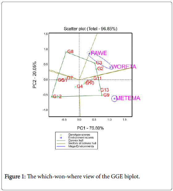
Polygon view of a biplot is the best way to visualize the interaction patterns between genotypes and environments, Yan and Kang [21]. They also noted that mega environment division must meet two requirements: first, there must be clear crossover genotype-by-location interactions that suggest different groups of locations, not environments, second any suggestions of mega-environments must be validated by joint analysis of multiple-year data. The polygon view of GGE biplot analysis of the present study is in agreement with Yan and Kang [21].
Figure 1 represents a polygon view of upland rice genotypes MET data. In this biplot, a polygon was formed by connecting the vertex genotypes with straight lines and the rest of the genotypes placed within the polygon. Genotypes 3, 8, 9 and 12 were the vertex genotypes which are the best or the poorest genotypes in some or all of the environments; for they were farthest from the origin of the biplot. From the polygon view of biplot analysis of MET data, the genotypes and test locations fell in four and two sections, respectively. The first section contains Woreta and Pawe which had the genotype 3 as the winner; the second section contains Metema with genotype 9 as the best yielder. This cross over GEI suggests that the target locations may be divided in to two mega environments (Woreta and Pawe as one and Metema as the other). No location fell in to the sector of vertex genotypes 8 and 12. This means that these vertex genotypes were not the winner in any of the locations; rather, they were likely to be the poorest genotypes in some or all of the locations.
Mean yield and stability performance of genotypes
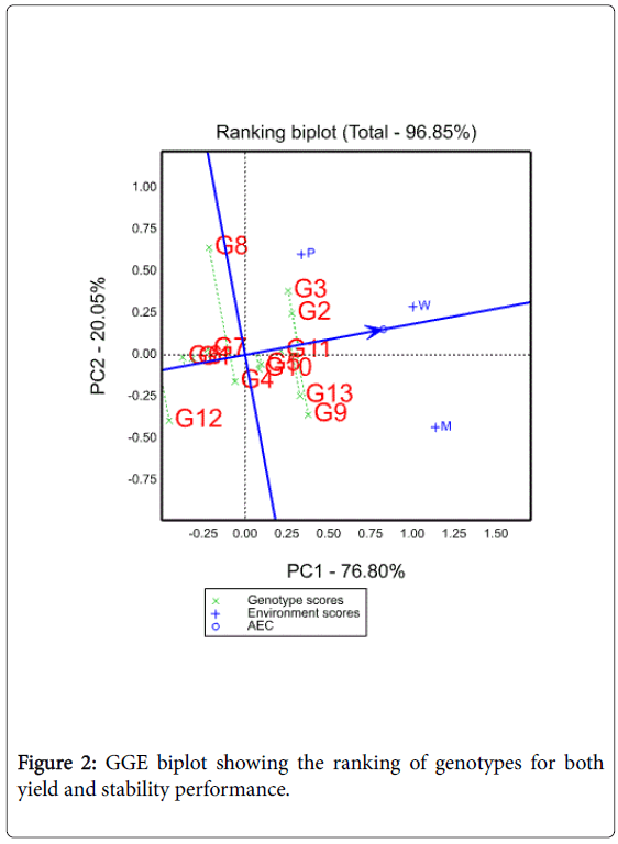
Yield performance and stability of genotypes were evaluated by an average environment coordination (AEC) method [22,23]. In this method, an average environment is defined by the average PC1 and PC2 scores of all environments, represented by a small circle (Figure 2). A line is then drawn to pass through this average environment and the biplot origin; which is called the average environment axis (AEA) and serves as the abscissa of the AEC. The ordinate of the AEC is the line that passes through the origin and is perpendicular to the AEC abscissa (Figure 2). Unlike the AEC abscissa, which has one direction, with the arrow pointing to greater genotype main effect, the AEC ordinate is indicated by double arrows, and either direction away from the biplot origin indicates greater GEI effect and reduced stability. Stability was reported to have lower heritability than mean performance [24] hence; it is useful only when considered jointly with mean performance.
In this study, in terms of mean yield performance , genotypes 2, 3, 5, 9, 10, 11 and 13 are found on the right side of the line with double arrows have yield performance greater than the grand mean while genotypes 1,4,6,7,8 and 12 are found on the left side of this line and had yields less than the grand mean. In terms of stability, the genotypes ranked as G11>G1>G6>G7>G5 >G10>G2>G4>G3>G12>G13>G9>G8 (Figure 2). Yan and Kang [21] noted that based on their grain yield and stability performance genotypes are classified in to three categories: (1) generally adapted, genotypes with high yield and high stability performance (2) specifically adapted, genotypes with high mean yield but low stability performance and (3) adapted nowhere, genotypes with low grain yield and low stability performance. In agreement with the findings of Eskridge [24], genotypes 11, 2 and 3 can be considered as genotypes with both high mean yield and high stability performance. On the other hand, genotypes with high yield but low stability were 9, 10 and 13 whereas genotypes with low yield and low stability were 8 and 12.
Evaluation of genotypes relative to an ideal genotype
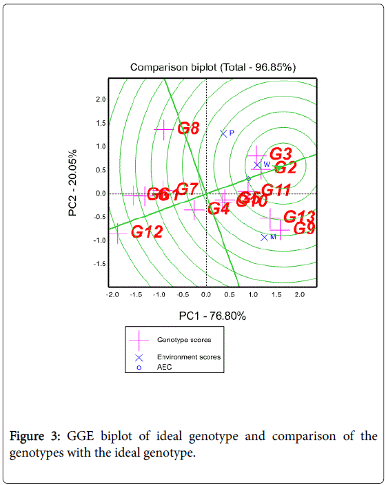
An ideal genotype should have the highest mean performance and be absolutely stable [25]. Such an ideal genotype is defined by having the greatest vector length of the high yielding genotypes with zero GEI, as represented by an arrow pointing to it (Figure 3). Although such an ideal genotype may not exist in reality, it can be used as a reference for genotype evaluation [25,26]. Thus, using the ideal genotype as the center, concentric circles were drawn to visualize the distance between each genotype and the ideal genotype. A genotype is more favorable if it is closer to the ideal genotype. Genotype 2 was near to the ideal genotype. Ranking of other genotypes based on the ideal genotype was 3>11>13>9>10>5. In other words, the lower yielding genotypes (4, 7, 8, 1, 6, and 12) were unfavorable because they are far from the ideal genotype.
Discriminating ability and representativeness of the test locations
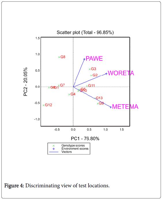
A test location which lacks discriminating ability provides no information about the cultivars [27,28]. Another equally important measure of a test location is its representativeness of the target environment. If a test location is not representative of the target environment, it is not only useless but also misleading since it may provide biased information about the tested cultivars [27]. The biplot as shown in Figure 4 helps to visualize the length of the environment vectors, which is proportional to the standard deviation within the respective locations and is a measure of the discriminating ability of the locations.
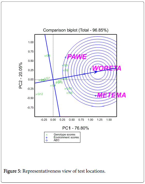
In this study, among the three testing locations Metema and Woreta were the most discriminating (informative) ones while Pawe was the least discriminating one. Figure 5 shows the average environment (represented by the small circle at the end of the arrow) which has the average coordinates of all test environments, and Average- Environment Axis (AEA) is the line that passes through the average environment and the biplot origin. Yan (2002:990-996) indicated that a test location that has a smaller angle with the AEA is more representative of other test locations. In the present study Woreta was found to be the most representative location while Pawe and Metema were the least representative ones (Figure 5).
Yan and Tinker [28] noted that test locations that are both discriminating and representative are good test environments for selecting generally adaptable genotypes while discriminating but nonrepresentative test environments are useful for selecting specifically adaptable genotypes if the target environments can be divided into mega-environments or they are useful for culling unstable genotypes if the target environment is a single mega-environment. In agreement with Yan and Tinker [28], Woreta was found to be both discriminating and representative for selecting generally adaptable genotypes while Metema was found to be discriminating to select specifically adapted genotypes.
Conclusion and Recommendation
The result of this study indicated that upland rice yield performance was influenced by the genotype effect followed by GEI and environment. The magnitude of genotype effect was found higher than both the GE interaction and environment effects indicating the significant contribution of the genotypes to grain yield. The majority of tested genotypes exhibited crossover type of GEI revealed by their differential rankings across test locations; however, three genotypes showed non-crossover type of GEI, indicating both types of interactions may happen. GGE biplot analysis allowed to visualize the “which-won-where’’ pattern of the genotypes, the ranking of genotypes based on both mean performance and stability, comparison of genotypes with the ideal genotype and the discriminating ability and representativeness of test locations.
The 13 upland rice genotypes showed variation for almost all measured characters. In terms of both mean grain yield and stability performance, there were desirable genotypes such as genotypes 3,2 and 11 while there were also genotypes with high grain yield but low stability such as genotype 9. The ideal-genotype biplot also confirmed that genotypes 2 followed by 3 and 11 were better genotypes in terms of mean yield and stability performance. Regarding testing locations, there exist two possible mega-environments. Among the testing locations, Woreta was identified an ideal location for selecting generally adaptable genotypes while Metema was good for selecting specifically adapted genotypes.
The result of this study can be considered as a driving force for the national rice breeding program of the country to execute multilocation yield trials at a number of potential upland rice growing areas of the country. So that demand driven, economical and mega environment oriented breeding strategy can be designed so that the effect of GEI can be either exploited or avoided as a result, sustainable rice production would be secured in the country.
Among the tested genotypes included in this study, three genotypes (2, 3 and 11) were selected and promoted to verification based on their better performance in terms of grain yield, stability, farmers’ preference and other desirable agronomic traits. Of which, genotype 2 has been officially released by the national variety release standing committee of the country with the common name NERICA-12 for large scale production.
References
- MoARD (Ministry of Agriculture and Rural Development) (2010) National Rice Research and Development Strategy of Ethiopia. Addis Ababa, Ethiopia, pp: 48.
- Kang MS, Aggarwal VD,Chirwa RM(2006) Adaptability and stability of bean cultivars as determined via yield-stability statistic and GGE biplot analysis. J Crop Sci Biotechnol 15: 97-120.
- Gauch HG, Zobel RW (1996) AMMI analysis of yield trials. In: Kang MS, Gauch HG (Editors) Genotype-by-environment interaction, Boca Raton, FL pp: 85-122.
- Yan W (2011) GGE biplot vs AMMI Graphs for Genotype x Environment Data Analysis. J Indian Soc Agric Stat 65: 181-193.
- Flores F, Moreno MT, Cubero JI (1998) A comparison of univariate and multivariate methods to analyze G × E interaction. Field Crops Res 56: 271–286.
- Gauch HG, Piepho HP, Annicchiarico P (2008) Statistical analysis of yield trials by AMMI and GGE: Further considerations. Crop Sci 48: 866-889.
- Yan W, Hunt LA, Sheng Q, Szlavnics Z (2000) Cultivar evaluation and mega-environment investigation based on the GGE biplot. Crop Sci 40: 597-605.
- Ding M, Tier B, Yan W (2007) Application of GGE biplot analysis to evaluate Genotype (G) Environment (E) and G × E interaction on P. radiata: a case study. Paper presented to Australasian Forest Genetics Conference Breeding for Wood Quality, Hobart, Tasmania, Australia.
- Fan XM, Kang MS, Chen H, Zhang Y, Tan J (2007) Yield stability of maize hybrids evaluated in multi-environment trials in Yunnan, China. AgronJ 99: 220–228.
- Balestre M, Souza JC, Von Pinho RG, Oliveira RL, Paes MVP (2009). Yield stability and adaptability of maize hybrids based on GGE biplot analysis characteristics. Crop Breed Appl Biotechnol 9: 226-234.
- Peterson CJ, Pfeiffer WH (1989) International winter wheat evaluation: Relationships among test sites based on cultivar performance. Crop Sci 29: 276-282.
- Gomez KA, Gomez AA (1984) Statistical procedures for agricultural research. 2nd edition. John Willey and Sons.
- Gabriel KR (1971) The biplot graphic display of matrices with application to principal component analysis. Biometrika 58: 453-467.
- Yan W (2001) GGEbiplot- a Windows application for graphiÂcal analysis of multi-environment trial data and other types of two-way data. Agron J 93:1111-1118.
- Taddesse L, Abebaw D, Sewagegne T, Desta A (2017) Evaluation of Performance and Yield Stability Analysis Based on AMMI and GGE Models in Introduced Upland Rice Genotypes Tested Across Northwest Ethiopia. IJRSAS 3: 17-24.
- Gauch GH, Zobel RW (1997) Interpreting mega-environments and targeting genotype crop Science. 37: 311-326.
- Farshadfar E, Hassan Z, Reza M (2011) Evaluation of phenotypic stability in chickpea genotypes using GGE-Biplot. Ann Biol Res 2: 282-292.
- Biswas PL, Nath UK, Ghosal S, Patwary AK (2012) Genotype-environment interaction and stability analysis of four fine rice varieties. Journal of Bangladesh Agricultural University. 10: 1–7.
- Matus-Cadiz MA, Hucl P, Perron CE, Tyler RT (2003). Genotype x environment interaction for grain color in hard white spring wheat. Crop Sci 43: 219-226
- Kaya Y, Akcura M, Taner S(2006) GGE-biplot analysis of multi-environment yield trials in bread wheat. Turk J Agric For. 30:325-337.
- Yan W, Kang MS (2003) GGE biplot analysis: A graphical tool for breeders, geneticists, and agronomists. CRC Press, Boca Raton, FL.
- Yan W, Hunt LA (2001) Interpretation of genotype x environment interaction for winter wheat yield in Ontario. Crop Sci 41: 19-25.
- Yan W (2002) Singular value partitioning for biplot analysis of multi-environment trial data. Agron J 94: 990–996.
- Eskridge KM (1996) Analysis of multiple environment trials using the probability of outperforming a check. In: Kang MS, Gauch, Jr. HG (Eds.), Genotype-by-environment interaction, CRC Press, Boca Raton, FL pp: 273-307.
- Karimizadehi R, Mohtasham MN, Sabaghn AA, Mahmood B, Roustami F, et al. (2013). GGE Biplot Analysis of Yield Stability in Multi-environment Trials of Lentil Genotypes under Rainfed Condition. Not Sci Biol 5: 256-262.
- Farshadfar E, Mohammadi MP, Maryam J (2012). Evaluation of phenotypic stability in bread wheat genotypes using GGE-biplot. International Journal of Agriculture and Crop Sci 4: 904-910.
- Dehghani H, Ebadi A, Yousefi A (2006) Biplot analysis of gnotype x environment interaction for barley yield in Iran. Agron J 98: 388-393.
- Yan W, Tinker NA (2006). Biplot analysis of multi-environment trial data: Principles and applications. Can J Plant Sci 86: 623-645.
Citation: Tariku S (2017) Evaluation of Upland Rice Genotypes and Mega Environment Investigation Based on GGE-Biplot Analysis. J Rice Res 5: 183. DOI: 10.4172/2375-4338.1000183
Copyright: © 2017 Tariku S. This is an open-access article distributed under the terms of the Creative Commons Attribution License, which permits unrestricted use, distribution, and reproduction in any medium, provided the original author and source are credited.
Select your language of interest to view the total content in your interested language
Share This Article
Recommended Journals
Open Access Journals
Article Tools
Article Usage
- Total views: 4743
- [From(publication date): 0-2017 - Jul 03, 2025]
- Breakdown by view type
- HTML page views: 3807
- PDF downloads: 936
